Factor rotation

• Unrotated factor solutions extract factors in the order of their variance extracted. 

• The first factor tends to be a general factor with almost every variable loading significantly, and it accounts for the largest amount of variance. The second and subsequent factors are then based on the residual amount of variance. Each accounts for successively smaller portions of variance. 

• The second and subsequent factors are then based on the residual amount of variance. Each accounts for successively smaller portions of variance. 

• The ultimate effect of rotating the factor matrix is to redistribute the variance from earlier factors to later ones to achieve a simpler, theoretically more meaningful factor pattern.

• The simplest case of rotation is an orthogonal factor rotation, in which the axes are maintained at 90 degrees. 

• It is also possible to rotate the axes and not retain the 90-degree angle between the reference axes. When not constrained to being orthogonal, the rotational procedure is called an oblique factor rotation. 

(Nguồn: https://devopedia.org/images/article/141/2168.1549391372.jpg)

ORTHOGONAL ROTATION METHODS

• In practice, the objective of all methods of rotation is to simplify the rows and columns of the factor matrix to facilitate interpretation. 
• In a factor matrix, columns represent factors, with each row corresponding to a variable’s loading across the factors.
• By simplifying the rows, we mean making as many values in each row as close to zero as possible (i.e., maximizing a variable’s loading on a single factor). 
• By simplifying the columns, we mean making as many values in each column as close to zero as possible (i.e., making the number of high loadings as few as possible). 
• Three major orthogonal approaches have been developed:

QUARTIMAX

• The ultimate goal of a QUARTIMAX rotation is to simplify the rows of a factor matrix that is, QUARTIMAX focuses on rotating the initial factor so that a variable loads high on one factor and as low as possible on all other factors. 

• In these rotations, many variables can load high or near high on the same factor because the technique centers on simplifying the rows

 VARIMAX

• In contrast to QUARTIMAX, the VARIMAX criterion centers on simplifying the columns of the factor matrix. 

• With the VARIMAX rotational approach, the maximum possible simplification is reached if there are only 1s and 0s in a column. That is, the VARIMAX method maximizes the sum of variances of required loadings of the factor matrix. 

• Recall that in QUARTIMAX approaches, many variables can load high or near high on the same factor because the technique centers on simplifying the rows. 

• With the VARIMAX rotational approach, some high loadings (i.e., close to –1 or +1) are likely, as are some loadings near 0 in each column of the matrix. The logic is that interpretation is easiest when the variable-factor correlations are (1) close to either +1 or –1, thus indicating a clear positive or negative association between the variable and the factor; or (2) close to 0, indicating a clear lack of association.

• This structure is fundamentally simple. Although the QUARTIMAX solution is analytically simpler than the VARIMAX solution, VARIMAX seems to give a clearer separation of the factors. 

• In general, Kaiser’s experiment indicates that the factor pattern obtained by VARIMAX rotation tends to be more invariant than that obtained by the QUARTIMAX method when different subsets of variables are analyzed. The VARIMAX method has proved successful as an analytic approach to obtaining an orthogonal rotation of factors.

EQUIMAX

• Approach is a compromise between the QUARTIMAX and VARIMAX approaches. Rather than concentrating either on simplification of the rows or on simplification of the columns, it tries to accomplish some of each. EQUIMAX has not gained widespread acceptance and is used infrequently.

OBLIQUE ROTATION METHODS 

• Oblique rotations are similar to orthogonal rotations, except that oblique rotations allow correlated factors instead of maintaining independence between the rotated factors.

• Where several choices are available among orthogonal approaches, however, most statistical packages typically provide only limited choices for oblique rotations. 
• For example, SPSS provides OBLIMIN; 
• SAS has PROMAX and ORTHOBLIQUE; 
• and BMDP provides DQUART, DOBLIMIN, and ORTHOBLIQUE. 

• The objectives of simplification are comparable to the orthogonal methods, with the added feature of correlated factors. With the possibility of correlated factors, the factor researcher must take additional care to validate obliquely rotated factors, because they have an additional way (nonorthogonality) of becoming specific to the sample and not generalizable, particularly with small samples or a low casesto-variable ratio.

SELECTING AMONG ROTATIONAL METHODS 

• No specific rules have been developed to guide the researcher in selecting a particular orthogonal or oblique rotational technique. 

• In most instances, the researcher simply utilizes the rotational technique provided by the computer program. 

• Most programs have the default rotation of VARIMAX, but all the major rotational methods are widely available. 

• However, no compelling analytical reason suggests favoring one rotational method over another. The choice of an orthogonal or oblique rotation should be made on the basis of the particular needs of a given research problem. 

(Nguồn: Hair et al, 2013)

 Nguồn thông tin:

• Hair, J. F., Black, W. C., Babin, B. J., & Anderson, R. E. (2013). Multivariate data analysis (8th ed.). Boston: Cengage.

Number of Factors to Extract

 Both factor analysis method ( known as common factor analysis and component analysis) are interested in the best linear combination of variables - best in the sense that the particular combination of original variables accounts for more of the variance in the data as a whole than any other linear combination of variables.

Therefore,

• the first factor may be viewed as the single best summary of linear relationships exhibited in the data.  

• The second factor is defined as the second-best linear combination of the variables, subject to the constraint that it is orthogonal to the first factor.  
• To be orthogonal to the first factor, the second factor must be derived from the variance remaining after the first factor has been extracted. 
• Thus, the second factor may be defined as the linear combination of variables that accounts for the most variance that is still unexplained after the effect of the first factor has been removed from the data.

• The process continues extracting factors accounting for smaller and smaller amounts of variance until all of the variance is explained.  

How many factors to extract or retain?

• The researcher must combine a conceptual foundation (How many factors should be in the structure?) with some empirical evidence (How many factors can be reasonably supported?). 

• An exact quantitative basis for deciding the number of factors to extract has not been developed. However, the following stopping criteria for the number of factors to extract are currently being utilized.

LATENT ROOT CRITERION

• This technique is simple to apply to either components analysis or common factor analysis.

• The rationale for the latent root criterion is that any individual factor should account for the variance of at least a single variable if it is to be retained for interpretation.

• With component analysis each variable contributes a value of 1 to the total eigenvalue.

• Thus, only the factors having latent roots or eigenvalues greater than 1 are considered significant; all factors with latent roots less than 1 are considered insignificant and are disregarded. 

• Using the eigenvalue for establishing a cutoff is most reliable when the number of variables is between 20 and 50.
• If the number of variables is less than 20, the tendency is for this method to extract a conservative number of factors (too few);
• whereas if more than 50 variables are involved, it is not uncommon for too many factors to be extracted.

A PRIORI CRITERION

• The a priori criterion is that the researcher already knows how many factors to extract before undertaking the factor analysis. 

• The researcher simply instructs the computer to stop the analysis when the desired number of factors has been extracted.

• This approach is useful when testing a theory or hypothesis about the number of factors to be extracted.

PERCENTAGE OF VARIANCE CRITERION

• The percentage of variance criterion is an approach based on achieving a specified cumulative percentage of total variance extracted by successive factors. 

• The purpose is to ensure practical significance for the derived factors by ensuring that they explain at least a specified amount of variance. No absolute threshold has been adopted for all applications. 

• However, in the natural sciences the factoring procedure usually should not be stopped until the extracted factors account for at least 95 percent of the variance or until the last factor accounts for only a small portion (less than 5%). 

• In contrast, in the social sciences, where information is often less precise, it is not uncommon to consider a solution that accounts for 60 percent of the total variance (and in some instances even less) as satisfactory.

• A variant of this criterion involves selecting enough factors to achieve a prespecified communality for each of the variables.
• If theoretical or practical reasons require a certain communality for each variable, then the researcher will include as many factors as necessary to adequately represent each of the original variables. 

• This approach differs from focusing on just the total amount of variance explained, which neglects the degree of explanation for the individual variables.

SCREE TEST CRITERION

•  With the component analysis factor model the later factors extracted contain both common and unique variance.

• Although all factors contain at least some unique variance, the proportion of unique variance is substantially higher in later factors.  

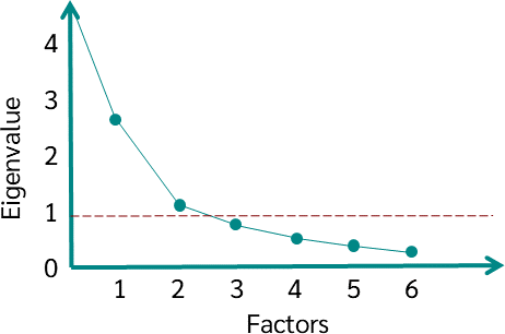
• The scree test is used to identify the optimum number of factors that can be extracted before the amount of unique variance begins to dominate the common variance structure

(Nguồn: https://datatab.net/assets/tutorial/PCA/en/Scree_test.png)

• The scree test is derived by plotting the latent roots against the number of factors in their order of extraction, and the shape of the resulting curve is used to evaluate the cutoff point.

HETEROGENEITY OF THE RESPONDENTS

• Shared variance among variables is the basis for both common and component factor models. An underlying assumption is that shared variance extends across the entire sample.

• If the sample is heterogeneous with regard to at least one subset of the variables, then the first factors will represent those variables that are more homogeneous across the entire sample. Variables that are better discriminators between the subgroups of the sample will load on later factors, many times those not selected by the criteria discussed previously.

• When the objective is to identify factors that discriminate among the subgroups of a sample, the researcher should extract additional factors beyond those indicated by the methods just discussed and examine the additional factors’ ability to discriminate among the groups. (Nghĩa là nếu mục tiêu là xác định nhân tố giúp phân biệt giữa các nhóm con trong một mẫu, thì bên cạnh các nhân tố đã được chọn ra theo các điều kiện bên trên, cần bổ sung thêm nhân tố giúp giải thích tốt sự khác biệt giữa các nhóm)

• If they prove less beneficial in discrimination, the solution can be run again and these later factors eliminated.

(Nguồn: Hair et al, 2013)

Nguồn thông tin:

• Hair, J. F., Black, W. C., Babin, B. J., & Anderson, R. E. (2013). Multivariate data analysis (8th ed.). Boston: Cengage.

Factor Extraction Method

 COMMON FACTOR ANALYSIS VERSUS COMPONENT ANALYSIS

The selection of one method over the other is based on two criteria:

• (1) the objectives of the factor analysis 
• (2) the amount of prior knowledge about the variance in the variables

Component analysis is used when the objective is to summarize most of the original information (variance) in a minimum number of factors for prediction purposes. 

In contrast, common factor analysis is used primarily to identify underlying factors or dimensions that reflect what the variables share in common. 

The most direct comparison between the two methods is by their use of the explained versus unexplained variance:

• Component analysis, also known as principal components analysis, considers the total variance and derives factors that contain small proportions of unique variance and, in some instances, error variance. 
• Common factor analysis, in contrast, considers only the common or shared variance, assuming that both the unique and error variance are not of interest in defining the structure of the variables. 

(Nguồn: Koch, A. F. (2016))

Component factor analysis is most appropriate when:

• Data reduction is a primary concern, focusing on the minimum number of factors needed to account for the maximum portion of the total variance represented in the original set of variables, and 

• Prior knowledge suggests that specific and error variance represent a relatively small proportion of the total variance

Common factor analysis is most appropriate when:

• The primary objective is to identify the latent dimensions or constructs represented in the original variables, and 

• The researcher has little knowledge about the amount of specific and error variance and therefore wishes to eliminate this variance.

Common factor analysis, with its more restrictive assumptions and use of only the latent dimensions (shared variance), is often viewed as more theoretically based. 

(Nguồn: Krishnan (2011).  )

Although theoretically sound, however, common factor analysis has several problems: 

• First, common factor analysis suffers from factor indeterminacy, which means that for any individual respondent, several different factor scores can be calculated from a single factor model result. No single unique solution is found, as in component analysis, but in most instances the differences are not substantial. 

• The second issue involves the calculation of the estimated communalities used to represent the shared variance. Sometimes the communalities are not estimable or may be invalid (e.g., values greater than 1 or less than 0), requiring the deletion of the variable from the analysis.

Tài liệu tham khảo

• Koch, A. F. (2016). Where is the link between direct, minimally guided and constructivist instruction? A new integrated model of constructivist teaching. EAPRIL 2016, 40. 
• Hair, J.F., Black, W.C., Babin, B.J. and Anderson, R.E. (2010) Multivariate Data Analysis. 7th Edition, Pearson, New York. 
• Krishnan, V. (2011). A comparison of principal components analysis and factor analysis for uncovering the early development instrument (EDI) domains. Unpublished manuscript, Early Child Development Mapping (ECMap) Project, Alberta, University of Alberta, Edmonton, Canada. 

Lịch sử của Factor Analysis

• Charles Spearman (1904): Được coi là người đặt nền móng cho phân tích nhân tố, SSpearman đưa ra lý thuyết hai yếu tố, trong đó thừa nhận yếu tố trí tuệ chung ('g') cùng với các yếu tố cụ thể dành riêng cho từng nhiệm vụ. Nghiên cứu của ông là nền tảng trong việc sử dụng phân tích nhân tố để hiểu khả năng nhận thức và kiểm tra trí thông minh của con người. 

(Nguồn: https://intelligenceccsw5.weebly.com/spearmans-g-factor.html)

• Thurstone (1930s): Thurstone mở rộng công trình của Spearman bằng cách phát triển phương pháp "multiple factor analysis". Ông không chỉ tìm kiếm một yếu tố chung mà còn khám phá nhiều yếu tố độc lập khác nhau đóng góp vào dữ liệu.\

(Nguồn: https://photoarchive.lib.uchicago.edu/db.xqy?one=apf1-09080.xml)

• Harold Hotelling (1930s) - Công trình của Hotelling về phân tích thành phần chính (PCA) có mối liên hệ đáng kể với phân tích nhân tố, vì PCA thường được sử dụng như một phương pháp để tính gần đúng các giải pháp phân tích nhân tố. Những đóng góp của ông cho thống kê đa biến đã ảnh hưởng đến nhiều ứng dụng khác nhau của phân tích nhân tố.

(Nguồn: https://magazine.amstat.org/blog/2018/10/29/sih-hotelling/)

• Raymond Cattell (1960s): Ông đề xuất "phân tích nhân tố khám phá" (EFA), một kỹ thuật cho phép phân tích mà không cần các giả định trước về cấu trúc của dữ liệu.

(Nguồn: https://psychologytheorists.wordpress.com/2016/05/26/raymond-cattell/)

• Karl Jöreskog (1970s): Jöreskog phát triển phương pháp "phân tích nhân tố khẳng định" (CFA), cho phép các nhà nghiên cứu kiểm định các mô hình lý thuyết đã được đề xuất trước đó về cấu trúc của dữ liệu. Jöreskog cũng đã đề xuất một phương pháp ước lượng hợp lý cực đại trong phân tích nhân tố. (Các phương pháp đáng tin cậy tương tự cũng được đề xuất bởi Gerhard Derflinger, Robert Jennrich và Stephen M. Robinson gần như cùng lúc.) Trong thời gian công tác tại the Educational Testing Service và giảng dạy tại đại học Princeton, Jöreskog đã đề xuất một mô hình tuyến tính để phân tích các cấu trúc hiệp phương sai, một đóng góp cơ bản cho mô hình phương trình cấu trúc (SEM).

Tài liệu tham khảo

• http://www.stats.org.uk/factor-analysis/Thurstone1931.pdf
• https://www.apadivisions.org/division-5/publications/score/2021/04/multidimensional-response
• https://rss.onlinelibrary.wiley.com/doi/abs/10.2307/2985729
• https://hal.science/hal-02557344/document

ASSUMPTIONS IN FACTOR ANALYSIS

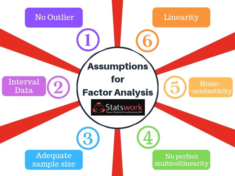
•  The critical assumptions underlying factor analysis are more conceptual than statistical.

Conceptual Issues

• The conceptual assumptions underlying factor analysis relate to the set of variables selected and the sample chosen. 

• A basic assumption of factor analysis is that some underlying structure does exist in the set of selected variables. The presence of correlated variables and the subsequent definition of factors do not guarantee relevance, even if they meet the statistical requirements. 

• It is the responsibility of the researcher to ensure that the observed patterns are conceptually valid and appropriate to study with factor analysis, because the technique has no means of determining appropriateness other than the correlations among variables. 
• For example, mixing dependent and independent variables in a single factor analysis and then using the derived factors to support dependence relationships is inappropriate.


• The researcher must also ensure that the sample is homogeneous with respect to the underlying factor structure. It is inappropriate to apply factor analysis to a sample of males and females for a set of items known to differ because of gender. 

• When the two subsamples (males and females) are combined, the resulting correlations and factor structure will be a poor representation of the unique structure of each group. Thus, whenever differing groups are expected in the sample, separate factor analyses should be performed, and the results should be compared to identify differences not reflected in the results of the combined sample.

Statistical Issues

• From a statistical standpoint, departures from normality, homoscedasticity, and linearity apply only to the extent that they diminish the observed correlations. 
• Only normality is necessary if a statistical test is applied to the significance of the factors, but these tests are rarely used. In fact, some degree of multicollinearity is desirable, because the objective is to identify interrelated sets of variables.
• Assuming the researcher has met the conceptual requirements for the variables included in the analysis, the next step is to ensure that the variables are sufficiently intercorrelated to produce representative factors. As we will see, we can assess this degree of interrelatedness from both overall and individual variable perspectives. 

The following are several empirical measures to aid in diagnosing the factorability of the correlation matrix.

• OVERALL MEASURES OF INTERCORRELATION
• In addition to the statistical bases for the correlations of the data matrix, the researcher must also ensure that the data matrix has sufficient correlations to justify the application of factor analysis. 




• If it is found that all of the correlations are low, or that all of the correlations are equal (denoting that no structure exists to group variables), then the researcher should question the application of factor analysis. 




• If visual inspection reveals no substantial number of correlations greater than .30, then factor analysis is probably inappropriate. The correlations among variables can also be analyzed by computing the partial correlations among variables. 

• If “true” factors exist in the data, the partial correlation should be small, because the variable can be explained by the variables loading on the factors. If the partial correlations are high, indicating no underlying factors, then factor analysis is inappropriate. 




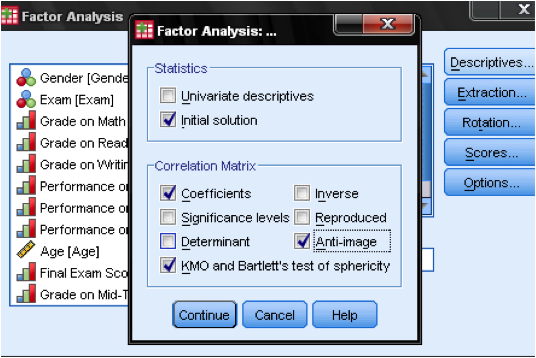
• A high partial correlation is one with practical and statistical significance, and a rule of thumb would be to consider partial correlations above .7 as high. SPSS and SAS provide the anti-image correlation matrix, which is just the negative value of the partial . Larger partial or anti-image correlations are indicative of a data matrix perhaps not suited to factor analysis.






(Nguồn: 

https://www.statisticssolutions.com)

• Another method of determining the appropriateness of factor analysis examines the entire correlation matrix. The Bartlett test of sphericity, a statistical test for the presence of correlations among the variables, is one such measure. It provides the statistical significance that the correlation matrix has significant correlations among at least some of the variables. The researcher should note, however, that increasing the sample size causes the Bartlett test to become more sensitive in detecting correlations among the variables

• A third measure to quantify the degree of intercorrelations among the variables and the appropriateness of factor analysis is the measure of sampling adequacy (MSA). This index ranges  from 0 to 1, reaching 1 when each variable is perfectly predicted without error by the other variables. The measure can be interpreted with the following guidelines: .80 or above, meritorious; .70 or above, middling; .60 or above, mediocre; .50 or above, miserable; and below .50, unacceptable. The MSA increases as (1) the sample size increases, (2) the average correlations increase, (3) the number of variables increases, or (4) the number of factors decreases. The researcher should always have an overall MSA value of above .50 before proceeding with the factor analysis. If the MSA value falls below .50, then the variablespecific MSA values (see the following discussion) can identify variables for deletion to achieve an overall value of .50

• VARIABLE-SPECIFIC MEASURES OF INTERCORRELATION

• In addition to a visual examination of a variable’s correlations with the other variables in the analysis, the MSA guidelines can be extended to individual variables. 

• The researcher should examine the MSA values for each variable and exclude those falling in the unacceptable range. In deleting variables, the researcher should first delete the variable with the lowest MSA and then recalculate the factor analysis.

• Continue this process of deleting the variable with the lowest MSA value under .50 until all variables have an acceptable MSA value. 

• Once the individual variables achieve an acceptable level, then the overall MSA can be evaluated and a decision made on continuance of the factor analysis.

Tài liệu gốc:

• Hair, J. F., Black, W. C., Babin, B. J., & Anderson, R. E. (2019). Multivariate data analysis (8th ed.). Boston: Cengage.

Sample Size in Factor Analysis

(Nguồn: 

https://www.qualtrics.com/experience-management/research/factor-analysis/ ) 

 

Hair, J. F. (2013). Multivariate data analysis.

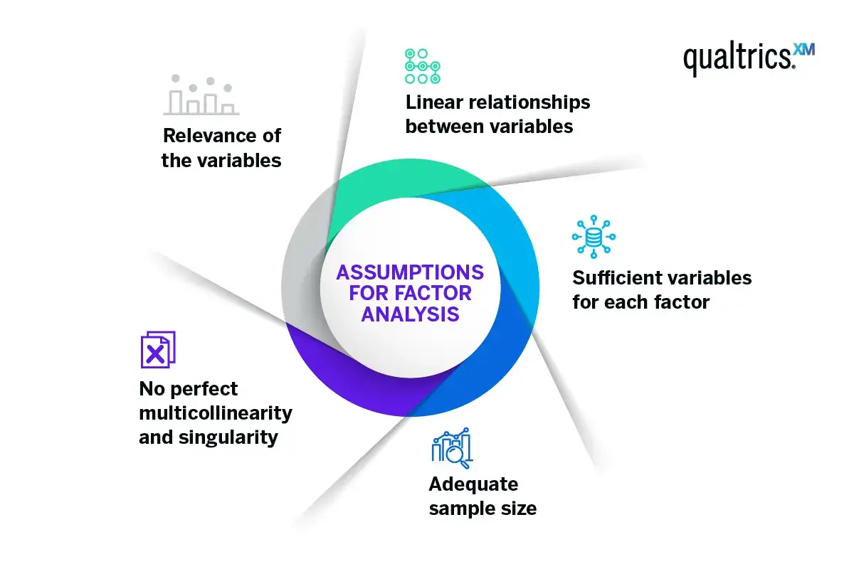
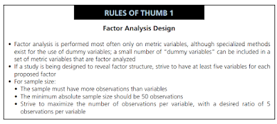
• Regarding the sample size question, the researcher generally would not factor analyze a sample of fewer than 50 observations, and preferably the sample size should be 100 or larger. 
• As a general rule, the minimum is to have at least five times as many observations as the number of variables to be analyzed, and the more acceptable sample size would have a 10:1 ratio.
• Some researchers even propose a minimum of 20 cases for each variable. One must remember, however, that 30 variables, for example, requires computing 435 correlations in the factor analysis. 
• At a .05 significance level, perhaps even 20 of those correlations would be deemed significant and appear in the factor analysis just by chance. The researcher should always try to obtain the highest cases-per-variable ratio to minimize the chances of overfitting the data.
•  In order to do so, the researcher may employ the most parsimonious set of variables, guided by conceptual and practical considerations, and then obtain an adequate sample size for the number of variables examined. 
• When dealing with smaller sample sizes and/or a lower cases-to-variable ratio, the researcher should always interpret any findings cautiously. 

Columbia University Mailman School of Public Health. Exploratory factor analysis. https://www.publichealth.columbia.edu

• Factor analysis has the following assumptions, which can be explored in more detail in the resources linked below:
• Sample size (e.g., 20 observations per variable)
• Level of measurement (e.g., the measurement/data scenarios above)
• Normality
• Linearity
• Outliers (factor analysis is sensitive to outliers)
• Factorability\

UCLA: Statistical Consulting Group. Factor analysis | SPSS Annotated Output.   https://stats.oarc.ucla.edu

• Factor analysis is a technique that requires a large sample size. 
• Factor analysis is based on the correlation matrix of the variables involved, and correlations usually need a large sample size before they stabilize. 
• Tabachnick and Fidell (2001, page 588) cite Comrey and Lee’s (1992) advise regarding sample size: 50 cases is very poor, 100 is poor, 200 is fair, 300 is good, 500 is very good, and 1000 or more is excellent.  
• As a rule of thumb, a bare minimum of 10 observations per variable is necessary to avoid computational difficulties.

The Analysis Factor. How big of a sample size do you need for factor analysis? https://www.theanalysisfactor.com

• For example, some authors use a criterion based on the total sample size:

• 100 subjects=sufficient if clear structure; more is better (Kline, 1994)
• 100 subjects=poor; 300 =good; 1000+ = excellent (Comrey & Lee, 1992)
• 300 subjects, though fewer works if correlations are high among variables (Tabachnik & Fidell, 2001)
• Others base it on a ratio of the number of cases to the number of variables involved in the factor analysis:

• 10-15 subjects per variable (Pett, Lackey, & Sullivan)
• 10 subjects per variable (Nunnally, 1978)
• 5 subjects per variable or 100 subjects, whichever is larger (Hatcher, 1994)
• 2 subjects per variable (Kline, 1994)

And then others base it on a ratio of cases to the number of factors: 20 subjects per factor (Arrindel & van der Ende, 1985).

Tài liệu gốc:

• https://www.publichealth.columbia.edu/research/population-health-methods/exploratory-factor-analysis
• https://www.theanalysisfactor.com/sample-size-needed-for-factor-analysis/
•  https://stats.oarc.ucla.edu
• 
  
• Hair, J. F., Black, W. C., Babin, B. J., Anderson, R. E., & Tatham, R. L. (2013). Multivariate Data Analysis (8th ed.). Edinburgh Gate, Harlow: Pearson  
• https://www.publichealth.columbia.edu

Rules of Thumb are not Rules

FACTOR ANALYSIS

INTRODUCTION

• Factor analysis is an interdependence technique whose primary purpose is to define the underlying structure among the variables in the analysis. 

• Factor analysis provides the tools for analyzing the structure of the interrelationships (correlations) among a large number of variables (e.g., test scores, test items, questionnaire responses) by defining sets of variables that are highly interrelated, known as factors. 

• These groups of variables (factors), which are by definition highly intercorrelated, are assumed to represent dimensions within the data. 

• If we are only concerned with reducing the number of variables, then the dimensions can guide in creating new composite measures. However, if we have a conceptual basis for understanding the relationships between variables, then the dimensions may actually have meaning for what they collectively represent. 

• In the latter case, these dimensions may correspond to concepts that cannot be adequately described by a single measure. We will see that factor analysis presents several ways of representing these groups of variables for use in other multivariate techniques. 

(Nguồn: https://statswork.com/blog/factor-analysis/)

• We should note at this point that factor analytic techniques can achieve their purposes from either an exploratory or confirmatory perspective. 

• For exploratory perspective, it is useful in searching for structure among a set of variables or as a data reduction method. In this perspective, factor analytic techniques “take what the data give you” and do not set any a priori constraints on the estimation of components or the number of components to be extracted.  

• For confirmatory perspective, researcher has preconceived thoughts on the actual structure of the data, based on theoretical support or prior research. In these instances, the researcher requires that factor analysis take a confirmatory approach—that is, assess the degree to which the data meet the expected structure. 

FACTOR ANALYSIS DECISION PROCESS

(Nguồn: Hair, 2013)

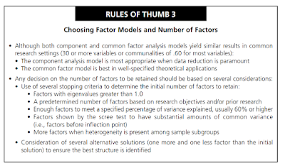
RULES OF THUMB 

(Nguồn: Hair, 2013)

Nguồn của thông tin

• Hair, J. F., Black, W. C., Babin, B. J., Anderson, R. E., & Tatham, R. L. (2013). Multivariate Data Analysis (8th ed.). Edinburgh Gate, Harlow: Pearson

Histograms

Histogram Basics

• Historams are constructed by binning the data and counting the number of observations in each bin. Common choices for the vertical scale are
• bin counts, or frequencies
• counts per unit, or densities
• The objective is usually to visualize the shape of the distribution.

A HISTOGRAM FOR COUNTING DATA

• The frequency of any particular x value is the number of times that value occurs in the data set. 
• The relative frequency of a value is the fraction or proportion of times the value occurs.
• A frequency distribution is a tabulation of the frequencies and/or relative frequencies.

Drawing histogram for counting data 

1. First, determine the frequency and relative frequency of each x value. 
2. Then mark possible x values on a horizontal scale.
3. Above each value, draw a rectangle whose height is the relative frequency (or alternatively, the frequency) of that value.

(Nguồn: https://think.design/services/data-visualization-data-design/histogram/)

This construction ensures that the area of each rectangle is proportional to the relative frequency of the value. 

A HISTOGRAM FOR MEASUREMENT DATA: EQUAL CLASS WIDTHS

• Constructing a histogram for measurement data (observations on a “measurement variable”) entails subdividing the measurement axis into a suitable number of class intervals or classes, such that each observation is contained in exactly one class.
• One potential difficulty is that occasionally an observation falls on a class boundary and therefore does not lie in exactly one interval. 
• We can use the convention that any observation falling on a class boundary will be included in the class to the right of the observation.

Drawing histogram for measurement data

1. Determine the frequency and relative frequency for each class. 
2. Mark the class boundaries on a horizontal measurement axis. 
3. Above each class interval, draw a rectangle whose height is the corresponding relative frequency (or frequency).

Note:

• There are no hard-and-fast rules concerning either the number of classes or the choice of classes themselves
• A reasonable rule of thumb is that the number of classes can be approximate the square root of the number of observations.
• Equal-width classes may not be a sensible choice if a data set “stretches out” to one side or the other. 
• Using a small number of equal-width classes results in almost all observations falling in just one or two of the classes. 
• If a large number of equal-width classes are used, many classes will have zero frequency.
• A sound choice is to use a few wider intervals near extreme observations and narrower intervals in the region of high concentration.

A HISTOGRAM FOR MEASUREMENT DATA: UNEQUAL CLASS WIDTHS

• After determining frequencies and relative frequencies, calculate the height of each rectangle using the formula 

rectangle height = relative frequency of the class : class width

• The resulting rectangle heights are usually called densities, and the vertical scale is the density scale. This prescription will also work when class widths are equal.

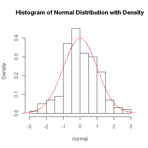
(Nguồn: https://datamining.togaware.com/survivor/Basic_Histogram0.html)

• When class widths are unequal, not using a density scale will give a picture with distorted areas.
• A density histogram does have one interesting property: the area of each rectangle is the relative frequency of the corresponding class. Because the sum of relative frequencies must be 1.0 (except for roundoff), the total area of all rectangles in a density histogram is l. 
• It is always possible to draw a histogram so that the area equals the relative frequency (this is true also for a histogram of counting data)—just use the density scale. 

Histogram Shapes

• A unimodal histogram is one that rises to a single peak and then declines. 
• A bimodal histogram has two different peaks.
• A histogram with more than two peaks is said to be multimodal
• A histogram is symmetric if the left half is a mirror image of the right half.
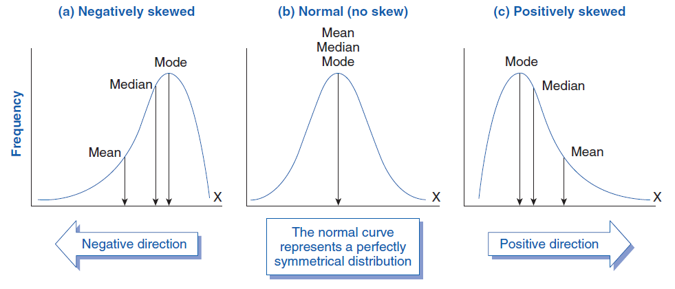
• A unimodal histogram is positively skewed if the right or upper tail is stretched out compared with the left or lower tail and negatively skewed if the stretching is to the left. 

(Nguồn: https://www.biologyforlife.com/skew.html)

Qualitative Data

• Both a frequency distribution and a histogram can be constructed when the data set is qualitative (categorical) in nature; in this case, “bar graph” is synonymous with “histogram.” 
• With such categorical data, the intervals above which rectangles are constructed should have equal width.

Nguồn của thông tin:

• Devore, J. L., Berk, K. N., & Carlton, M. A. (2012). Modern mathematical statistics with applications (Vol. 285). New York: Springer.

 

Statistics

 Một số định nghĩa về thống kê

• Statistics is the science concerned with developing and studying methods for collecting, analyzing, interpreting and presenting empirical data.  (https://www.stat.uci.edu/what-is-statistics/)

• Statistics is a branch of applied mathematics that involves the collection, description, analysis, and inference of conclusions from quantitative data. (Investopia)

(Nguồn: https://www.investopedia.com/terms/s/statistics.asp)

• Statistics is the study of the collection, analysis, interpretation, presentation, and organization of data. In other words, it is a mathematical discipline to collect, summarize data. Also, we can say that statistics is a branch of applied mathematics. (https://byjus.com/maths/statistics/)

• Statistics is the discipline that concerns the collection, organization, analysis, interpretation, and presentation of data. (https://en.wikipedia.org/wiki/Statistics)

• Statistics, the science of collecting, analyzing, presenting, and interpreting data.  (https://www.britannica.com/science/statistics)

• Statistics has a double meaning. First, Statistics is concerned with scientific methods for collecting, organizing, summarizing, presenting, and analyzing data, as well as drawing valid conclusions and making relevant decisions on the basis of such analysis. In another sense, statistics is used to denote the data themselves. We can speak of economic statistics, geophysical statistics, employment statistics, accident statistics, financial statistics, population statistics, etc. To say that data are statistics, the data sets must be capable of being compared, and must be representative and coherent, and must have been systematically produced so that relevant or significant comparisons or computations can be made. Not all data are statistical data, i.e., able to be analyzed by a statistical method. (https://www.sciencedirect.com/topics/mathematics/statistics)

• Statistics is also a term that refers to the practice of collecting, analysing, interpreting and communicating data. It is the science of interacting with data. (Australian Bureau of Statistics)

• Statistics: the science of using information discovered from collecting, organizing, and studying numbers (https://dictionary.cambridge.org/dictionary/english/statistics)

• Statistics: a branch of mathematics dealing with the collection, analysis, interpretation, and presentation of masses of numerical data (https://www.merriam-webster.com/dictionary/statistics)

• Statistics is the technology of extracting information, illumination and understanding from data, often in the face of uncertainty.  (https://www.thebritishacademy.ac.uk/blog/what-is-statistics/)

• Stats is a branch of mathematics concerned with the study of information that is expressed in numbers. (https://www.collinsdictionary.com/dictionary/english/stats) 

• Statistics is the science of collecting and analyzing numerical data in large quantities, especially for the purpose of inferring proportions as a whole from those in a representative sample. (https://scse.d.umn.edu/what-math)

• Statistics is a way to understand the data that is collected about us and the world.  (https://www.statisticshowto.com/statistic/)

• Statistics is a branch of mathematics that involves collecting, describing, and gaining insights from data. (https://articles.outlier.org/what-is-statistics)

(Nguồn: https://qph.cf2.quoracdn.net)

Những kết luận có thể rút ra từ các định nghĩa trên

• Statistics liên quan đến việc phân tích dữ liệu, bao gồm thu thập, mô tả, tổ chức, tóm tắt và giải thích các thông tin của dữ liệu đó.

• Statistics được xem là một nhánh của toán học, cụ thể là toán ứng dụng.

• Statistics dựa trên dữ liệu thực nghiệm, nghĩa là thống kê liên quan đến các quan sát và đo lường trong thế giới thực hơn là các hệ thống lý thuyết.

• Statistics  thực hiện việc đưa ra các suy luận hoặc kết luận dựa trên phân tích dữ liệu,  diễn giải kết quả để rút ra những thông tin hoặc những hiểu biết có ý nghĩa.

• Statistics phân tích dữ liệu để có thêm hiểu biết trong tình huống không chắc chắn hoặc có biến động trong dữ liệu. 

Nguồn tham khảo khác

• https://magazine.amstat.org/blog/2022/10/01/what-is-statistics/
• https://www.jstor.org/stable/1652319?seq=1
• 
  

Hornbostel-Sachs

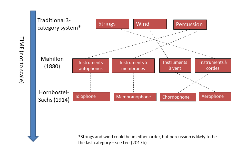
Hệ phân loại Hornbostel-Sachs là một hệ thống phân loại khoa học các nhạc cụ, được đề xuất lần đầu vào năm 1914 bởi hai nhà âm nhạc học người Áo là Erich Moritz von Hornbostel và Curt Sachs. Hệ thống này dựa trên hệ phân loại đã có từ trước của nhà văn hóa học và ngôn ngữ học Victor-Charles Mahillon, người đã cố gắng phân loại các nhạc cụ trong bộ sưu tập của mình cho Bảo tàng Công cụ Âm nhạc Hoàng gia ở Brussels.

(Nguồn: https://www.isko.org/cyclo/hornbostel1.jpg)

Hệ thống Hornbostel-Sachs chia nhạc cụ thành bốn nhóm chính dựa trên cách thức âm thanh được tạo ra:

• Bộ dây (Chordophones): Những nhạc cụ này tạo ra âm thanh nhờ vào sự rung động của các dây đàn. Chúng được phân loại thành các loại nhạc cụ dây có thể gảy, búng, hoặc cào, như đàn guitar, đàn violin.

• Bộ kèn (Aerophones): Âm thanh được tạo ra khi không khí chảy qua một khoang, bao gồm cả kèn thổi và các loại sáo. Nhóm này bao gồm các nhạc cụ như kèn trombone, kèn trumpet, và sáo.

(Nguồn: https://i.pinimg.com)

• Nhạc cụ gõ (Membranophones): Nhạc cụ này tạo âm thanh khi một màng (da trống) được gõ hoặc rung động. Ví dụ điển hình là trống, bongo.

(Nguồn)

• Nhạc cụ tự âm (Idiophones): Trong nhóm này, chính thân của nhạc cụ rung động để tạo ra âm thanh mà không cần dây đàn hoặc màng. Ví dụ về nhạc cụ tự âm bao gồm chuông, xylophone.

(Nguồn: https://i.pinimg.com)

Nguồn tham khảo:

• https://anhtran95blog.wordpress.com/2018/08/21/he-thong-phan-loai-nhac-cu-cac-bo-nhac-cu-va-he-thong-sachs-hornbostel/
• https://www.isko.org/cyclo/hornbostel
• 
  

Fractal Geometry

Fractal là một thuật ngữ do nhà Toán học Mandelbrot đưa ra khi ông khảo sát những hình hoặc những hiện tượng trong thiên nhiên không có đặc trưng về độ dài. Fractal thể hiện sự gần giống nhau về hình dạng của các hình thể kích cỡ khác nhau. 

(Nguồn: https://www.fotoview.nl/UltimateFractal/images/image1.png)

Hình học fractal (Fractal Geometry) là một nhánh của toán học nghiên cứu các đối tượng phức tạp có tính tự lặp lại ở mọi quy mô. Khái niệm này được biểu diễn qua các cấu trúc tự tương tự, nghĩa là một phần nhỏ của fractal là bản sao thu nhỏ của toàn bộ. Chiều fractal (fractal dimension), một khái niệm trung tâm trong hình học fractal, đo lường sự phức tạp của fractal bằng cách xem xét cách độ dài, diện tích hoặc thể tích của nó thay đổi khi được đo ở các tỷ lệ khác nhau.

(Nguồn: https://galileounbound.files.wordpress.com/2020/12/fractals.jpg?w=2400)

Lịch sử ra đời

Dù các đối tượng tự tương tự đã được nhận biết từ lâu trong thiên nhiên, khái niệm về fractal chỉ thực sự được định hình bởi nhà toán học Benoit Mandelbrot vào năm 1975. Mandelbrot đã giới thiệu thuật ngữ "fractal" để mô tả những cấu trúc hình học không thể được mô tả hoàn toàn bằng hình học truyền thống. Ông đã khám phá ra rằng fractals có thể cung cấp một mô hình toán học để diễn tả nhiều hiện tượng tự nhiên phức tạp, như đường bờ biển, tuyết, và cây cối.

Ứng dụng

Fractals được ứng dụng rộng rãi trong nhiều lĩnh vực khác nhau. 

• Trong khoa học máy tính, chúng được sử dụng để nén dữ liệu và tạo đồ họa máy tính, cung cấp một phương pháp hiệu quả để lưu trữ hình ảnh phức tạp.

(Nguồn: https://static.vecteezy.com/system/)

• Trong khoa học tự nhiên, fractals giúp giải thích các cấu trúc phức tạp và mô hình hóa các hệ thống động lực như mây, dãy núi, hoặc hệ thống mạch máu. 

    

(Nguồn: https://incubator.rockefeller.edu/wp-content/uploads/2013/03/fractals-in-nature-1.png)

• Trong y học, hình ảnh fractal được sử dụng để phân tích các mô hình của các cấu trúc sinh học như phổi và mạch máu, giúp chẩn đoán và nghiên cứu bệnh lý. 

(Nguồn: https://genomeden.com/wp-content/uploads/2023/07/lungs-fractal.webp)

• Ngoài ra, các nguyên tắc fractal cũng được áp dụng trong kinh tế học để mô hình hóa các thị trường tài chính, nhận dạng các xu hướng và mô hình biến động giá.

Tài liệu tham khảo

• https://www.cs.uic.edu/~jbell/CourseNotes/ComputerGraphics/SpecialTopics.html
• https://galileo-unbound.blog/2020/12/26/a-short-history-of-fractal-dimension/
• https://www.wahl.org/fe/HTML_version/link/FE4W/c4.htm
• https://repository.vnu.edu.vn/bitstream/VNU_123/13045/1/7.pdf

Hurst exponent

 Số mũ Hurst, còn được gọi là chỉ số Hurst (ký hiệu là 𝐻), là một tham số thống kê được sử dụng để đánh giá tính tự tương quan trong chuỗi thời gian hoặc cấu trúc tự tương tự của dữ liệu. Nó được đặt theo tên của Harold Edwin Hurst ((1880–1978), một kỹ sư người Anh, người đã sử dụng chỉ số này trong nghiên cứu về chu kỳ của lũ lụt ở sông Nile để dự đoán lũ lụt và hạn hán.

Số mũ Hurst được sử dụng để xác định liệu một chuỗi dữ liệu có tính chất "memory" hay không, tức là liệu các giá trị trong quá khứ có ảnh hưởng đến các giá trị tương lai. Nó cũng giúp phân biệt ba loại hành vi khác nhau trong chuỗi thời gian:

• Chuyển động Brown (Brownian Motion ): 𝐻>0,5. Khi H lớn hơn 0,5, chuỗi dữ liệu cho thấy tính tự tương quan dương, nghĩa là xu hướng trong quá khứ sẽ tiếp tục diễn ra trong tương lai. Điều này thường được gọi là "tính động lượng" trong các tài sản tài chính.
• Bước ngẫu nhiên  (Random walk): 𝐻=0.5. Khi H = 0.5, chuỗi dữ liệu biểu hiện như một bước ngẫu nhiên, không có tự tương quan giữa các điểm dữ liệu.
• Chuỗi quy về giá trị trung bia2nh (Mean-Reverting): 𝐻<0,5. Khi  𝐻 nhỏ hơn 0.5, chuỗi cho thấy tính tự tương quan âm, tức là xu hướng hiện tại có khả năng sẽ đảo ngược trong tương lai. Điều này có thể được nhìn thấy trong các quá trình dao động, nơi một biến động lớn có thể theo sau bởi biến động ngược lại.

Chỉ số Hurst thường được tính bằng phương pháp p R/S (Rescaled Range). Đây là một cách phổ biến để ước lượng số mũ Hurst trong phân tích thống kê của chuỗi thời gian tài chính và các chuỗi thời gian khác. 

(Nguồn: https://community.esri.com/t5/python-questions/hurst-exponent/td-p/390500)

Nguồn tham khảo:

• https://community.esri.com/t5/python-questions/hurst-exponent/td-p/390500
• https://blog.quantinsti.com/hurst-exponent/
• https://c.mql5.com/forextsd/forum/170/hurst_exponent_and_financial_market_predictability.pdf

Cowles Commission

Cowles Commission for Research in Economics, hoặc đơn giản là Cowles Commission, là một tổ chức nghiên cứu kinh tế được thành lập vào năm 1932 bởi Alfred Cowles tại Colorado Springs. Sau đó, tổ chức này chuyển đến Chicago vào năm 1939 và liên kết với Đại học Chicago cho đến năm 1955. Năm 1955, các chuyên viên nghiên cứu chuyên nghiệp của Cowles Commission đã chấp nhận bổ nhiệm tại Yale và cùng với các thành viên khác của Khoa Kinh tế Yale, đã thành lập đội ngũ nghiên cứu của tổ chức hiện tại - The Cowles Foundation.

(Nguồn: https://www.hetwebsite.net/het/schools/cowles.htm)

Quỹ Cowles cung cấp hỗ trợ cho nghiên cứu và các hoạt động liên quan đến nghiên cứu thông qua các Chương trình Nghiên cứu trong bảy lĩnh vực cốt lõi mà Cowles quan tâm: Thuật toán, Dữ liệu và Thiết kế Thị trường; Kinh tế lượng; Lý thuyết kinh tế; Tổ chức công nghiệp; Thương mại quốc tế; Lao động và Kinh tế công cộng; và Kinh tế vĩ mô. Cowles Commission nổi tiếng với việc đưa ra những phương pháp nghiên cứu kinh tế tiên tiến và là một trong những ngôi trường phái tiên phong trong lĩnh vực kinh tế học toán học. Trong suốt thập kỷ 1940 và 1950, Cowles Commission đã thu hút sự quan tâm của nhiều nhà kinh tế học hàng đầu và đã sản sinh ra một loạt các nghiên cứu đột phá. Một trong những nghiên cứu nổi bật của Cowles Commission là việc phát triển và ứng dụng các phương pháp thống kê và toán học vào nghiên cứu kinh tế. Đây là nơi mà các nhà nghiên cứu như Tjalling Koopmans, Jacob Marschak, Kenneth Arrow, và Herbert Simon đã phát triển các phương pháp mới trong lĩnh vực học kinh tế, bao gồm cả mô hình toán học của hành vi kinh tế, lý thuyết quyết định và lý thuyết trò chơi.

Cowles Commission Computational Laboratory in Chicago. 

(Nguồn: https://www.researchgate.net/figure/)

Một số nhà nghiên cứu nổi bật của tổ chức này:

• Tjalling Koopmans: Tjalling Koopmans lnổi tiếng với công trình về lý thuyết tối ưu và ứng dụng của nó vào kinh tế học. Ông đã đoạt Giải Nobel Kinh tế vào năm 1975 vì đóng góp của mình vào lĩnh vực này.

• Jacob Marschak: Jacob Marschak là một nhà kinh tế học người Ukraine, là một trong những thành viên sáng lập của Cowles Commission. Ông đã đóng góp quan trọng vào phát triển lý thuyết quyết định và thống kê kinh tế.

• Kenneth Arrow: Kenneth Arrow là một nhà kinh tế học và toán học nổi tiếng, được biết đến với công trình về lý thuyết quyết định và lý thuyết trò chơi. Ông đã được trao Giải Nobel Kinh tế vào năm 1972.

• Herbert Simon: Herbert Simon là một nhà kinh tế học, nhà tâm lý học và nhà khoa học máy tính nổi tiếng. Ông đã đóng góp vào nhiều lĩnh vực, bao gồm lý thuyết quyết định, lý thuyết tổ chức và trí tuệ nhân tạo. Ông cũng đã nhận Giải Nobel Kinh tế vào năm 1978.

• Trygve Haavelmo: Trygve Haavelmo là một nhà kinh tế học người Na Uy, nổi tiếng với công trình về phương pháp kinh tế toán học. Ông đã đoạt Giải Nobel Kinh tế vào năm 1989 vì đóng góp của mình vào phân tích kinh tế định lượng.

• James Tobin: là một trong những nhà kinh tế học hàng đầu của thế kỷ 20 và đã nhận Giải Nobel Kinh tế vào năm 1981 vì công trình của mình về lý thuyết tài chính và chính sách tiền tệ. Một trong những đóng góp nổi bật của Tobin là việc phát triển mô hình đầu tư và tiêu dùng. Ông đã đưa ra lý thuyết về quyết định đầu tư của doanh nghiệp và tác động của chính sách tiền tệ lên các quyết định đầu tư này. Đồng thời, ông cũng nghiên cứu về tác động của thuế và các biện pháp chính sách khác đối với tiêu dùng và đầu tư. Tobin cũng được biết đến với "mô hình Tobin's Q", một khái niệm quan trọng trong lĩnh vực tài chính. Mô hình này phản ánh mối quan hệ giữa giá trị thị trường của một công ty và giá trị thực sự của tài sản của công ty đó. Nó đã có ảnh hưởng sâu rộng đến nghiên cứu và thực tiễn trong lĩnh vực tài chính và đầu tư.

Nguồn tham khảo:

• https://www.hetwebsite.net/het/schools/cowles.htm
• https://cowles.yale.edu/sites/default/files/2022-08/history-cowles.pdf
• https://cowles.yale.edu/about

xtabond2

•    xtabond2 can fit two closely related dynamic panel data models.
• The first is the Arellano-Bond (1991) estimator, which is also available with     xtabond, though without the two-step standard error correction described below.  It is sometimes called "difference GMM."
• The second is an augmented version outlined by Arellano and Bover (1995) and fully developed by Blundell and Bond (1998).  It is known as "system GMM." 

• Roodman (2009) provides a pedagogic introduction to linear GMM, these estimators, and xtabond2.

•  The estimators are designed for dynamic "small-T, large-N" panels that may contain fixed effects and - separate from those fixed effects - idiosyncratic errors that are heteroskedastic and correlated within but not across individuals. 

Mô hình: 

 y_it = x_it * b_1 + w_it * b_2 + u_it      i=1,...,N;     t=1,...,T

    u_it = v_i + e_it,

 where

• v_i are unobserved individual-level effects;
• e_it are the observation-specific errors;
• x_it is a vector of strictly exogenous covariates (ones dependent on neither current nor past e_it);
• w_it is a vector of predetermined covariates (which may include the lag of y) and endogenous covariates, all of which may be correlated with the v_i (Predetermined variables are potentially correlated with past errors.  Endogenous ones are potentially correlated with past and present errors.);
• b_1 and b_2 are vectors of parameters to be estimated;
•  and E[v_i]=E[e_it]=E[v_i*e_it]=0, and E[e_it*e_js]=0 for each i, j, t, s, i<>j.

• First-differencing the equation removes the v_i, thus eliminating a potential source of omitted variable bias in estimation.

• However, differencing     variables that are predetermined but not strictly exogenous makes them endogenous since the w_it in some D.w_it = w_it - w_i,t-1 is correlated with the e_i,t-1 in D.e_it.

• Following Holt-Eakin, Newey, and Rosen (1988), Arellano and Bond (1991) develop a Generalized Method of Moments estimator     that instruments the differenced variables that are not strictly exogenous with all their available lags in levels. 

•  A problem with the original Arellano-Bond estimator is that lagged levels are poor instruments for first differences if the variables are close to a random walk.

• Arellano and Bover (1995) describe how, if the original equation in levels is added to the system, additional instruments can be brought to bear to increase efficiency.  In this equation, variables in levels are instrumented with suitable lags of their own first differences.

• The assumption needed is that these differences are uncorrelated with the unobserved country effects.  Blundell and Bond show that this assumption in turn depends on a more precise one about initial conditions.

• The Mata version also includes the option to use the forward orthogonal deviations transform instead of first differencing.  Proposed by Arellano and Bover (1995) the orthogonal deviations transform, rather than subtracting the previous observation, subtracts the average of all available future observations. The result is then multiplied by a scale factor chosen to yield the nice but relatively unimportant property that if the original e_it     are i.i.d., then so are the transformed ones (see Arellano and Bover (1995) and Roodman (2009)). 

• Like differencing, taking orthogonal deviations  removes fixed effects.  Because lagged observations of a variable do not enter the formula for the transformation, they remain orthogonal to the     transformed errors (assuming no serial correlation), and available as instruments.

• In fact, for consistency, the software stores the orthogonal deviation of an observation one period late, so that, as with differencing, observations for period 1 are missing and, for an instrumenting variable w, w_i,t-1 enters the formula for the transformed observation stored at i,t.  With this move, exactly the same lags of variables are valid as instruments under the two transformations.

• On balanced panels, GMM estimators based on the two transforms return numerically identical coefficient estimates, holding the instrument set fixed (Arellano and Bover 1995).  But orthogonal deviations has the virtue of preserving sample size in panels with gaps.  If some e_it is missing, for example, neither D.e_it nor D.e_i,t+1 can be computed.  But the orthogonal deviation can be computed for every complete observation except the last for each individual.  (First differencing can do no better since it must drop the first observation for each individual.) Note that "difference GMM"  is still called that even when orthogonal deviations are used.  We will refer to the equation in differences or orthogonal deviations as the transformed equation.  In system GMM with orthogonal deviations, the levels or untransformed equation is still instrumented with differences as described above.

• xtabond2 reports the Arellano-Bond test for autocorrelation, which is applied to the differenced residuals in order to purge the unobserved and perfectly autocorrelated v_i.  AR(1) is expected in first differences, because D.e_i,t = e_i,t - e_i,t-1 should correlate with D.e_i,t-1 = e_i,t-1 -     e_i,t-2 since they share the e_i,t-1 term.  So to check for AR(1) in levels, look for AR(2) in differences, on the idea that this will detect the relationship between the e_i,t-1 in D.e_i,t and the e_i,t-2 in D.e_i,t-2.  This reasoning does not work for orthogonal deviations, in which the     residuals for an individual are all mathematically interrelated, thus contaminated from the point of view of detecting AR in the e_it.  So the test is run on differenced residuals even after estimation in deviations.  Autocorrelation indicates that lags of the dependent variable (and any other variables used as instruments that are not strictly exogenous), are in fact endogenous, thus bad instruments.  For example, if there is AR(s), then y_i,t-s would be correlated with e_i,t-s, which would be correlated with D.e_i,t-s, which would be correlated with D.e_i,t.

• xtabond2 also reports tests of over-identifying restrictions--of whether the instruments, as a group, appear exogenous.  
• For one-step, non-robust estimation, it reports the Sargan statistic, which is the minimized value of the one-step GMM criterion function.  The Sargan statistic is not robust to heteroskedasticity or autocorellation.  
• So for one-step, robust estimation (and for all two-step estimation), xtabond2 also reports the Hansen J statistic, which is the minimized value of the two-step GMM criterion function, and is robust.   
• xtabond2 still reports the Sargan statistic in these cases because the J test has its own problem: it can be greatly weakened by instrument proliferation.   
• The Mata version goes further, reporting  difference-in-Sargan statistics (really, difference-in-Hansen statistics, except in one-step robust estimation), which test for whether subsets of instruments are valid.   
• To be precise, it reports one test for each group of instruments defined by an ivstyle() or gmmstyle() option (explained below).  So replacing gmmstyle(x y) in a command line with gmmstyle(x) gmmstyle(y) will yield the same estimate but distinct difference-in-Sargan/Hansen tests.  
• In addition, including the split suboption in a gmmstyle() option in system GMM splits an instrument group in two for difference-in-Sargan/Hansen purposes, one each for the transformed equation and levels equations.  This is especially useful for testing the     instruments for the levels equation based on lagged differences of the dependent variable, which are the most suspect in system GMM and the subject of the "initial conditions" in the title of Blundell and Bond (1998).   
• In the same vein, in system GMM, xtabond2 also tests all the GMM-type instruments for the levels equation as a group.  All of these tests, however, are weak when the instrument count is high.
•  Difference-in-Sargan/Hansen tests are are computationally intensive since they involve re-estimating the model for each test; the nodiffsargan option is available to prevent them.

• As linear GMM estimators, the Arellano-Bond and Blundell-Bond estimators have one- and two-step variants.  But though two-step is asymptotically more efficient, the reported two-step standard errors tend to be severely downward biased (Arellano and Bond 1991; Blundell and Bond 1998).  To compensate, xtabond2 makes available a finite-sample correction to the two-step covariance matrix derived by Windmeijer (2005).  This can make two-step robust estimations more efficient than one-step robust, especially for system GMM.

• The syntax of xtabond2 differs substantially from that of xtabond and xtdpdsys.  xtabond2 almost completely decouples specification of regressors from specification of instruments.  As a result, most variables used will appear twice in an xtabond2 command line.

• xtabond2 requires the initial varlist of the command line to include all regressors except for the optional constant term, be they strictly exogenous, predetermined, or endogenous.  Variables used to form instruments then appear in gmmstyle() or ivstyle() options after the comma.  The result is a loss of parsimony, but fuller control over the instrument matrix.  Variables can be used as the basis for "GMM-style" instrument sets without being included as regressors, or vice versa.

Nguồn tài liệu:

• Roodman, D. 2009. How to do xtabond2: An introduction to difference and system GMM in Stata. Stata Journal 9(1): 86-136.