OUTLIERS (Hair, 2013)

Outliers are observations with a unique combination of characteristics identifiable as distinctly different from the other observations. It is judged to be an unusually high or low value on a variable or a unique combination of values across several variables that make the observation stand out from the others. 

In assessing the impact of outliers, we must consider the practical and substantive considerations:

• From a practical standpoint, outliers can have a marked effect on any type of empirical analysis.
• In substantive terms, the outlier must be viewed in light of how representative it is of the population

Outliers cannot be categorically characterized as either beneficial or problematic, but instead must be viewed within the context of the analysis and should be evaluated by the types of information they may provide. 

• When beneficial, outliers—although different from the majority of the sample— may be indicative of characteristics of the population that would not be discovered in the normal course of analysis. 
• In contrast, problematic outliers are not representative of the population, are counter to the objectives of the analysis, and can seriously distort statistical tests. Owing to the varying impact of outliers, it is imperative that the researcher examine the data for the presence of outliers and ascertain their type of influence. Additionally, outliers should be placed in a framework particularly suited for assessing the influence of individual observations and determining whether this influence is helpful or harmful.

METHODS OF DETECTING OUTLIERS

• Univariate Detection. 

The univariate identification of outliers examines the distribution of observations for each variable in the analysis and selects as outliers those cases falling at the outer ranges (high or low) of the distribution. The primary issue is establishing the threshold for designation of an outlier. The typical approach first converts the data values to standard scores, which have a mean of 0 and a standard deviation of 1. Because the values are expressed in a standardized format, comparisons across variables can be made easily.

(Nguồn: https://ai-ml-analytics.com/outlier-detection/)

 

In either case, the researcher must recognize that a certain number of observations may occur  normally in these outer ranges of the distribution. The researcher should strive to identify only those truly distinctive observations and designate them as outliers. 

• Bivariate Detection. 

In addition to the univariate assessment, pairs of variables can be assessed jointly through a scatterplot. Cases that fall markedly outside the range of the other observations will be seen as isolated points in the scatterplot. To assist in determining the expected range of observations in this two-dimensional portrayal, an ellipse representing a bivariate normal distribution’s confidence interval (typically set at the 90% or 95% level) is superimposed over the scatterplot. This ellipse provides a graphical portrayal of the confidence limits and facilitates identification of the outliers. A variant of the scatterplot is termed the influence plot, with each point varying in size in relation to its influence on the relationship.

(Nguồn: https://ouzhang.me/blog/outlier-series/outliers-part4/)

 

Each of these methods provides an assessment of the uniqueness of each observation in relationship to the other observation based on a specific pair of variables. A drawback of the bivariate method in general is the potentially large number of scatterplots that arise as the number of variables increases. For three variables, it is only three graphs for all pairwise comparisons. But for five variables, it takes 10 graphs, and for 10 variables it takes 45 scatterplots! As a result, the researcher should limit the general use of bivariate methods to specific relationships between variables, such as the relationship of the dependent versus independent variables in regression. The researcher can then examine the set of scatterplots and identify any general pattern of one or more observations that would result in their designation as outliers.

• Multivariate Detection. 

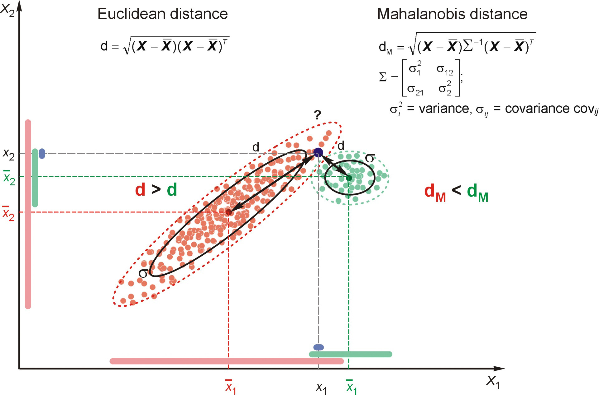
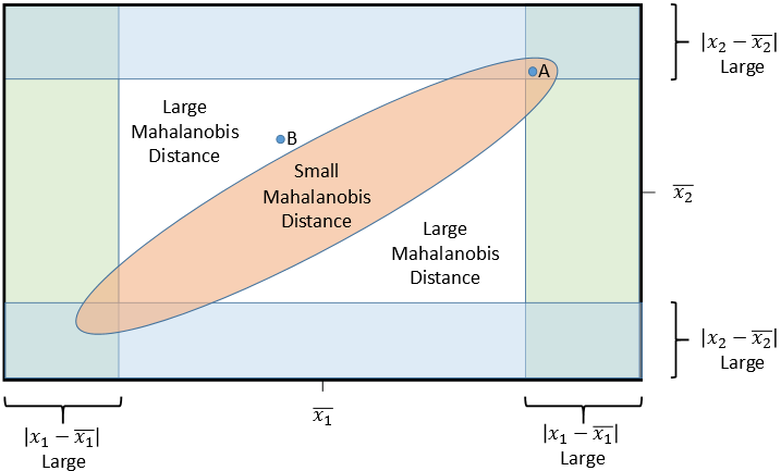
Because most multivariate analyses involve more than two variables, the bivariate methods quickly become inadequate for several reasons. First, they require a large number of graphs, as discussed previously, when the number of variables reaches even moderate size. Second, they are limited to two dimensions (variables) at a time. Yet when more than two variables are considered, the researcher needs a means to objectively measure the multidimensional position of each observation relative to some common point.

(Nguồn: https://blogs.sas.com/content/iml/2019/03/25/geometry-multivariate-univariate-outliers.html)

 

This issue is addressed by the Mahalanobis D2 measure, a multivariate assessment of each observation across a set of variables. This method measures each observation’s distance in multidimensional space from the mean center of all observations, providing a single value for each observation no matter how many variables are considered. Higher D2 values represent observations farther removed from the general distribution of observations in this multidimensional space. This method, however, also has the drawback of only providing an overall assessment, such that it provides no insight as to which particular variables might lead to a high D2 value.

(Nguồn: Hair, 2013)

 

RETENTION OR DELETION OF THE OUTLIER 

After the outliers are identified, profiled, and categorized, the researcher must decide on the retention or deletion of each one. Many philosophies among researchers offer guidance as to how to deal with outliers. Our belief is that they should be retained unless demonstrable proof indicates that they are truly aberrant and not representative of any observations in the population. If they do portray a representative element or segment of the population, they should be retained to ensure generalizability to the entire population. As outliers are deleted, the researcher runs the risk of improving the multivariate analysis but limiting its generalizability. If outliers are problematic in a particular technique, many times they can be accommodated in the analysis in a manner in which they do not seriously distort the analysis.

Nguồn:

•  Hair, J. F. (2009). Multivariate data analysis.

A RECAP OF THE MISSING VALUE ANALYSIS (Hair, 2013)

(Nguồn:https://www.researchgate.net/publication/329398079_The_Sin_of_Missing_Data_Is_All_Forgiven_by_Way_of_Imputation/figures?lo=1 )

 

Evaluation of the issues surrounding missing datain the data set can be summarized in four conclusions:

• The missing data process is MCAR. 

All of the diagnostic techniques support the conclusion that no systematic missing data process exists, making the missing data MCAR (missing completely at random). Such a finding provides two advantages to the researcher. First, it should not involve any hidden impact on the results that need to be considered when interpreting the results. Second, any of the imputation methods can be applied as remedies for the missing data. Their selection need not be based on their ability to handle nonrandom processes, but instead on the applicability of the process and its impact on the results.  

• Imputation is the most logical course of action. 

Even given the benefit of deleting cases and variables, the researcher is precluded from the simple solution of using the complete case method, because it results in an inadequate sample size. Some form of imputation is therefore needed to maintain an adequate sample size for any multivariate analysis.

• Imputed correlations differ across techniques.

 When estimating correlations among the variables in the presence of missing data, the researcher can choose from four commonly employed techniques: the complete case method, the all-available information method, the mean substitution method, and the EM method. The researcher is faced in this situation, however, with differences in the results among these methods. The all-available information, mean substitution, and EM approaches lead to generally consistent results. Notable differences, however, are found between these approaches and the complete information approach. Even though the complete information approach would seem the most “safe” and conservative, in this case it is not recommended due to the small sample used (only 26 observations) and its marked differences from the other two methods. The researcher should, if necessary, choose among the other approaches.

• Multiple methods for replacing the missing data are available and appropriate. 

Mean substitution is one acceptable means of generating replacement values for the missing data. The researcher also has available the regression and EM imputation methods, each of which give reasonably consistent estimates for most variables. The presence of several acceptable methods also enables the researcher to combine the estimates into asingle composite, hopefully mitigating any effects strictly due to one of the methods.

Nguồn: 

•  Hair, J. F. (2009). Multivariate data analysis.

Missing Data (Hair, 2013)

 A Four-Step Process for Identifying Missing Data

Nguồn: Hair, J. F. (2009). Multivariate data analysis.

STEP 1: DETERMINE THE TYPE OF MISSING DATA 

The first step in any examination of missing data is to determine the type of missing data involved. Here the researcher is concerned whether the missing data are part of the research design and under the control of the researcher or whether the “causes” and impacts are truly unknown. Let’s start with the missing data that are part of the research design and can be handled directly by the researcher.

• Ignorable Missing Data:  The justification for designating missing data as ignorable is that the missing data process is operating at random (i.e., the observed values are a random sample of the total set of values, observed and missing) or explicitly accommodated in the technique used. There are three instances in which a researcher most often encounters ignorable missing data.

• The first example encountered in almost all surveys and most other data sets is the ignorable missing data process resulting from taking a sample of the population rather than gathering data from the entire population.  In these instances, the missing data are those observations in a population that are not included when taking a sample. The purpose of multivariate techniques is to generalize from the sample observations to the entire population, which is really an attempt to overcome the missing data of observations not in the sample. The researcher makes these missing data ignorable by using probability sampling to select respondents. Probability sampling enables the researcher to specify that the missing data process leading to the omitted observations is random and that the missing data can be accounted for as sampling error in the statistical procedures. Thus, the missing data of the nonsampled observations are ignorable.

• A second instance of ignorable missing data is due to the specific design of the data collection process. Certain nonprobability sampling plans are designed for specific types of analysis that accommodate the nonrandom nature of the sample. Much more common are missing data due to the design of the data collection instrument, such as through skip patterns where respondents skip sections of questions that are not applicable 

• A third type of ignorable missing data occurs when the data are censored. Censored data are observations not complete because of their stage in the missing data process. A typical example is an analysis of the causes of death. Respondents who are still living cannot provide complete information (i.e., cause or time of death) and are thus censored. 

       

STEP 2: DETERMINE THE EXTENT OF MISSING DATA

The primary issue in this step of the process is to determine whether the extent or amount of missing data is low enough to not affect the results, even if it operates in a nonrandom manner. If it is sufficiently low, then any of the approaches for remedying missing data may be applied. If the missing data level is not low enough, then we must first determine the randomness of the missing data process before selecting a remedy (step 3).

How Much Missing Data Is Too Much?

Nguồn: Hair, J. F. (2009). Multivariate data analysis.

            Assessing the Extent and Patterns of Missing Data. 

The most direct means of assessing the extent of missing data is by tabulating (1) the percentage of variables with missing data for each case and (2) the number of cases with missing data for each variable. This simple process identifies not only the extent of missing data, but any exceptionally high levels of missing data that occur for individual cases or observations. The researcher should look for any nonrandom patterns in the data, such as concentration of missing data in a specific set of questions, attrition in not completing the questionnaire, and so on. Finally, the researcher should determine the number of cases with no missing data on any of the variables, which will provide the sample size available for analysis if remedies are not applied.

f it is determined that the extent is acceptably low and no specific nonrandom patterns appear, then the researcher can employ any of the imputation techniques (step 4) without biasing the results in any appreciable manner. If the level of missing data is too high, then the researcher must consider specific approaches to diagnosing the randomness of the missing data processes (step 3) before proceeding to apply a remedy 

 

    Deletions Based on Missing Data

Nguồn: Hair, J. F. (2009). Multivariate data analysis.

Imputation of Missing Data

Nguồn: Hair, J. F. (2009). Multivariate data analysis.

STEP 3: DIAGNOSE THE RANDOMNESS OF THE MISSING DATA PROCESSES

   Levels of Randomness of the Missing Data Process

• Missing At Random, or MAR

Missing data are termed missing at random (MAR) if the missing values of Y depend on X,

but not on Y. In other words, the observed Y values represent a random sample of the actual Y values for each value of X, but the observed data for Y do not necessarily represent a truly random sample of all Y values. Even though the missing data process is random in the sample, its values are not generalizable to the population. Most often, the data are missing randomly within subgroups, but differ in levels between subgroups. The researcher must determine the factors determining the subgroups and the varying levels between groups.

• Missing Completely At Random, or MCAR

A higher level of randomness is termed missing completely at random (MCAR). In these instances the observed values of Y are truly a random sample of all Y values, with no underlying process that lends bias to the observed data. In simple terms, the cases with missing data are indistinguishable from cases with complete data.

 

Only MCAR allows for the use of any remedy desired. The distinction between these two levels is in the generalizability to the population

 Diagnostic Tests for Levels of Randomness. 

• The first diagnostic assesses the missing data process of a single variable Y by forming two groups: observations with missing data for Y and those with valid values of Y. Statistical tests are then performed to determine whether significant differences exist between the two groups on other variables of interest. Significant differences indicate the possibility of a nonrandom missing data process.

• A second approach is an overall test of randomness that determines whether the missing data can be classified as MCAR. This test analyzes the pattern of missing data on all variables and compares it with the pattern expected for a random missing data process. If no significant differences are found, the missing data can be classified as MCAR. If significant differences are found, however, the researcher must use the approaches described previously to identify the specific missing data processes that are nonrandom.

As a result of these tests, the missing data process is classified as either MAR or MCAR, which then determines the appropriate types of potential remedies. Even though achieving the level of MCAR requires a completely random pattern in the missing data, it is the preferred type because it allows for the widest range of potential remedies.

STEP 4: SELECT THE IMPUTATION METHOD

Imputation is the process of estimating the missing value based on valid values of other variables and/or cases in the sample. The objective is to employ known relationships that can be identified in the valid values of the sample to assist in estimating the missing values. However, the researcher should carefully consider the use of imputation in each instance because of its potential impact on the analysis 

Comparison of Imputation Techniques for Missing Data

Nguồn: Hair, J. F. (2009). Multivariate data analysis.

All of the imputation methods discussed in this section are used primarily with metric variables; nonmetric variables are left as missing unless a specific modeling approach is employed. Nonmetric variables are not amenable to imputation because even though estimates of the missing data for metric variables can be made with such values as a mean of all valid values, no comparable measures are available for nonmetric variables. As such, nonmetric variables require an estimate of a specific value rather than an estimate on a continuous scale. It is different to estimate a missing value for a metric variable, such as an attitude or perception—even income—than it is to estimate the respondent’s gender when missing.

Nguồn: 

• Nguồn: Hair, J. F. (2009). Multivariate data analysis

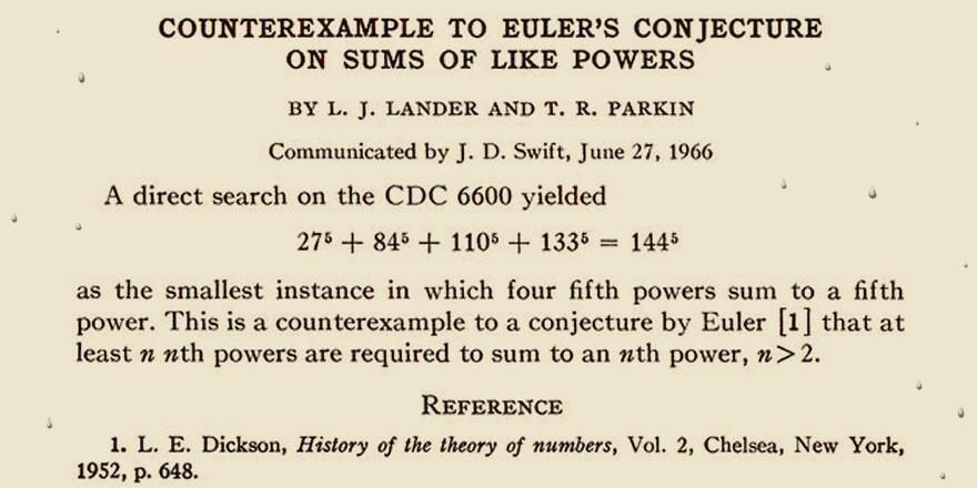
Bài báo Toán học ngắn nhất

 

(Nguồn: https://www.openculture.com/2015/04/shortest-known-paper-in-a-serious-math-journal.html)

Nguồn tham khảo: 

• https://www.openculture.com/2015/04/shortest-known-paper-in-a-serious-math-journal.html
• https://www.numberphile.com/videos/the-shortest-ever-papers

A CLASSIFICATION OF MULTIVARIATE TECHNIQUES (Hair, 2013)

 

• A dependence technique may be defined as one in which a variable or set of variables is identified as the dependent variable to be predicted or explained by other variables known as independent variables. An example of a dependence technique is multiple regression analysis.

Một số kỹ thuật của "dependence technique" 

(Nguồn: Hair, J. F. (2009). Multivariate data analysis. )

• In contrast, an interdependence technique is one in which no single variable or group of variables is defined as being independent or dependent. Rather, the procedure involves the simultaneous analysis of all variables in the set. Factor analysis is an example of an interdependence technique. 

TYPES OF MULTIVARIATE TECHNIQUES

1. Principal components and common factor analysis
2. Multiple regression and multiple correlation
3.  Multiple discriminant analysis and logistic regression
4. Canonical correlation analysis
5. Multivariate analysis of variance and covariance
6. Conjoint analysis
7. Cluster analysis
8. Perceptual mapping, also known as multidimensional scaling
9. Correspondence analysis
10. Structural equation modeling and confirmatory factor analysis

Principal Components and Common Factor Analysis

Factor analysis, including both principal component analysis and common factor analysis, is a statistical approach that can be used to analyze interrelationships among a large number of variables and to explain these variables in terms of their common underlying dimensions (factors). The objective is to find a way of condensing the information contained in a number of original variables into a smaller set of variates (factors) with a minimal loss of information. By providing an empirical estimate of the structure of the variables considered, factor analysis becomes an objective basis for creating summated scales. 

 

Multiple Regression

Multiple regression is the appropriate method of analysis when the research problem involves a single metric dependent variable presumed to be related to two or more metric independent variables. The objective of multiple regression analysis is to predict the changes in the dependent variable in response to changes in the independent variables. This objective is most often achieved through the statistical rule of least squares.

 

Multiple Discriminant Analysis and Logistic Regression

Multiple discriminant analysis (MDA) is the appropriate multivariate technique if the single dependent variable is dichotomous (e.g., male–female) or multi-chotomous (e.g., high–medium–low) and therefore nonmetric. As with multiple regression, the independent variables are assumed to be metric. Discriminant analysis is applicable in situations in which the total sample can be divided into groups based on a nonmetric dependent variable characterizing several known classes. The primary objectives of multiple discriminant analysis are to understand group differences and to predict the likelihood that an entity (individual or object) will belong to a particular class or group based on several metric independent variables 

Logistic regression models, often referred to as logit analysis, are a combination of multiple regression and multiple discriminant analysis. This technique is similar to multiple regression analysis in that one or more independent variables are used to predict a single dependent variable. What distinguishes a logistic regression model from multiple regression is that the dependent variable is nonmetric, as in discriminant analysis. The nonmetric scale of the dependent variable requires differences in the estimation method and assumptions about the type of underlying distribution, yet in most other facets it is quite similar to multiple regression. Thus, once the dependent variable is correctly specified and the appropriate estimation technique is employed, the basic factors considered in multiple regression are used here as well. Logistic regression models are distinguished from discriminant analysis primarily in that they accommodate all types of independent variables (metric and nonmetric) and do not require the assumption of multivariate normality. However, in many instances, particularly with more than two levels of the dependent variable, discriminant analysis is the more appropriate technique.

 

Canonical Correlation

Canonical correlation analysis can be viewed as a logical extension of multiple regression analysis. With canonical analysis the objective is to correlate simultaneously several metric dependent variables and several metric independent variables. Whereas multiple regression involves a single dependent variable, canonical correlation involves multiple dependent variables. The underlying principle is to develop a linear combination of each set of variables (both independent and dependent) in a manner that maximizes the correlation between the two sets. Stated in a different manner, the procedure involves obtaining a set of weights for the dependent and independent variables that provides the maximum simple correlation between the set of dependent variables and the set of independent variables. 

Multivariate Analysis of Variance and Covariance

Multivariate analysis of variance (MANOVA) is a statistical technique that can be used to simultaneously explore the relationship between several categorical independent variables (usually referred to as treatments) and two or more metric dependent variables. As such, it represents an extension of univariate analysis of variance (ANOVA). Multivariate analysis of covariance (MANCOVA) can be used in conjunction with MANOVA to remove (after the experiment) the effect of any uncontrolled metric independent variables (known as covariates) on the dependent variables. The procedure is similar to that involved in bivariate partial correlation, in which the effect of a third variable is removed from the correlation. MANOVA is useful when the researcher designs an experimental situation (manipulation of several nonmetric treatment variables) to test hypotheses concerning the variance in group responses on two or more metric dependent variables.

Conjoint Analysis

Conjoint analysis is an emerging dependence technique that brings new sophistication to the evaluation of objects, such as new products, services, or ideas. The most direct application is in new product or service development, allowing for the evaluation of complex products while maintaining a realistic decision context for the respondent. The market researcher is able to assess the importance of attributes as well as the levels of each attribute while consumers evaluate only a few product profiles, which are combinations of product levels.

Assume a product concept has three attributes (price, quality, and color), each at three possible levels (e.g., red, yellow, and blue). Instead of having to evaluate all 27 (3 * 3 * 3) possible combinations, a subset (9 or more) can be evaluated for their attractiveness to consumers, and the researcher knows not only how important each attribute is but also the importance of each level (e.g., the attractiveness of red versus yellow versus blue). Moreover, when the consumer evaluations are completed, the results of conjoint analysis can also be used in product design simulators, which show customer acceptance for any number of product formulations and aid in the design of the optimal product.

Cluster Analysis

Cluster analysis is an analytical technique for developing meaningful subgroups of individuals or objects. Specifically, the objective is to classify a sample of entities (individuals or objects) into a small number of mutually exclusive groups based on the similarities among the entities. In cluster analysis, unlike discriminant analysis, the groups are not predefined. Instead, the technique is used to identify the groups. 

Perceptual Mapping

In perceptual mapping (also known as multidimensional scaling), the objective is to transform consumer judgments of similarity or preference (e.g., preference for stores or brands) into distances represented in multidimensional space. If objects A and B are judged by respondents as being the most similar compared with all other possible pairs of objects, perceptual mapping techniques will  position objects A and B in such a way that the distance between them in multidimensional space is smaller than the distance between any other pairs of objects. The resulting perceptual maps show the relative positioning of all objects, but additional analyses are needed to describe or assess which attributes predict the position of each object.

As an example of perceptual mapping, let’s assume an owner of a Burger King franchise wants to know whether the strongest competitor is McDonald’s or Wendy’s. A sample of customers is given a survey and asked to rate the pairs of restaurants from most similar to least similar. The results show that the Burger King is most similar to Wendy’s, so the owners know that the strongest competitor is the Wendy’s restaurant because it is thought to be the most similar. Follow-up analysis can identify what attributes influence perceptions of similarity or dissimilarity. 

Correspondence Analysis

Correspondence analysis is a recently developed interdependence technique that facilitates the perceptual mapping of objects (e.g., products, persons) on a set of nonmetric attributes. Researchers are constantly faced with the need to “quantify the qualitative data” found in nominal variables. Correspondence analysis differs from the interdependence techniques discussed earlier in its ability to accommodate both nonmetric data and nonlinear relationships. In its most basic form, correspondence analysis employs a contingency table, which is the cross-tabulation of two categorical variables. It then transforms the nonmetric data to a metric level and performs dimensional reduction (similar to factor analysis) and perceptual mapping. 

Correspondence analysis provides a multivariate representation of interdependence for nonmetric data that is not possible with other methods. As an example, respondents’ brand preferences can be cross-tabulated on demographic variables (e.g., gender, income categories, occupation) by indicating how many people preferring each brand fall into each category of the demographic variables. Through correspondence analysis, the association, or “correspondence,” of brands and the distinguishing characteristics of those preferring each brand are then shown in a two- or three-dimensional map of both brands and respondent characteristics. Brands perceived as similar are located close to one another. Likewise, the most distinguishing characteristics of respondents preferring each brand are also determined by the proximity of the demographic variable categories to the brand’s position.

Structural Equation Modeling and Confirmatory Factor Analysis

Structural equation modeling (SEM) is a technique that allows separate relationships for each of a set of dependent variables. In its simplest sense, structural equation modeling provides the appropriate and most efficient estimation technique for a series of separate multiple regression equations estimated simultaneously. It is characterized by two basic components: (1) the structural model and (2) the measurement model. The structural model is the path model, which relates independent to dependent variables. In such situations, theory, prior experience, or other guidelines enable the researcher to distinguish which independent variables predict each dependent variable. Models discussed previously that accommodate multiple dependent variables—multivariate analysis of variance and canonical correlation—are not applicable in this situation because they allow only a single relationship between dependent and independent variables. 

The measurement model enables the researcher to use several variables (indicators) for a single independent or dependent variable. For example, the dependent variable might be a concept represented by a summated scale, such as self-esteem. In a confirmatory factor analysis the researcher can assess the contribution of each scale item as well as incorporate how well the scale measures the concept (reliability). The scales are then integrated into the estimation of the relationships between dependent and independent variables in the structural model. This procedure is similar to performing a factor analysis (discussed in a later section) of the scale items and using the factor scores in the regression.

Nguồn: 

• Hair, J. F. (2009). Multivariate data analysis.

Visual Summaries of book "Introduction to Statistics and Data Analysis - Heumann et al"

 Descriptive Data Analysis

Summary of Tests for Continuous and Ordinal Variables

(Part a)

(Nguồn b)

(Part c)

Summary of Tests for Nominal Variables

Nguồn: Heumann et al., Introduction to Statistics and Data Analysis, Springer International Publishing Switzerland, 2016.

DOI 10.1007/978-3-319-46162-5

Lịch năm 2024 trùng với lịch 1996

 Năm 2024 có lịch trùng với năm 1996

(Nguồn)

Điều này có thể lý giải bằng quy tắc toán học. Năm 2024 và năm 1996 có cùng 2 đặc điểm: ngày 1-1 rơi vào thứ Hai và đều là năm nhuận (tháng 2 có ngày 29).

Làm một phép tính đơn giản: lấy 365 (số ngày trong năm thường) chia cho 7 (số ngày trong tuần) dư 1. Vậy nên sau mỗi năm, ngày dương lịch sẽ tăng một thứ. Ví dụ: ngày 1-1 của năm 2020 là thứ Hai, sang 2021 là thứ Ba.

Sau 7 năm, lịch lại trùng nhau về thứ trong tuần. Tuy nhiên, vì trong năm nhuận có thêm 1 ngày nên quá trình "tăng một thứ" nêu trên lại được đẩy nhanh 1 ngày. Điều này khiến cho chu kỳ lặp lại diễn ra chỉ sau 5 hoặc 6 năm (tùy vào việc có 1 hay 2 ngày nhuận chen vào giữa).

Sau khi kết hợp 4 năm nhuận với 7 ngày một tuần, hai năm nhuận cách nhau 28 năm sẽ có lịch giống nhau. Như vậy, năm 1996 cũng không phải là năm duy nhất có lịch giống y hệt năm 2024. Theo trang Time and Date, còn 5 năm nhuận khác sẽ lịch giống năm 2024, đó là 1940, 1968, 2052, 2080 và 2120.

Tham khảo:

• https://tuoitre.vn/lich-nam-2024-trung-lich-nam-1996-co-la-khong-20240106080036351.htm
• https://muctim.tuoitre.vn/lich-nam-2024-va-1996-giong-nhau-su-ky-la-co-quy-tac-101240106121720021.htm

Dividend-smoothing policies

Dividend-smoothing policies - chính sách làm mượt cổ tức

(Nguồn: https://fastercapital.com/keyword/dividend-smoothing.html)

Làm mượt cổ tức là khi doanh nghiệp giữ cho tỷ lệ tăng trưởng dòng cổ tức tiền mặt chi trả hàng năm ở một mức cố định. 

Có 5 lý thuyết tạo cơ sở cho doanh nghiệp áp dụng chính sách làm mượt cổ tức.

• Lý thuyết đại diện (Agency theory): Việc duy trì dòng cổ tức tăng trưởng đều đặn qua hàng năm giúp giảm thiểu mâu thuẫn giữa cổ đông (tức  người sở hữu doanh nghiệp) và ban quản trị. Một mức cổ tức được định sẵn sẽ giúp tạo thuận lợi cho việc điều hành hoạt động kinh doanh của công ty để tạo lợi nhuận.

• Lý thuyết bất cân xứng thông tin (Asymmetric information theory). Do hiện tượng bất cân xứng thông tin xảy ra giữa nhà đầu tư và ban lãnh đạo doanh nghiệp, những người điều hành có khả năng dự báo chính xác hơn về kết quả hoạt động kinh doanh của doanh nghiệp trong tương lai. Vì vậy, những doanh nghiệp có kết quả kinh doanh biến động mạnh hoặc có xu hướng đi xuống trong tương lai thường có xu hướng làm mượt cổ tức. Khi đó, việc chi trả cổ tức đều đặn kết hợp với một số nghiệp vụ kế toán có thể tạo ra cảm giác an toàn cho nhà đầu tư về kết quả kinh doanh của doanh nghiệp. 

• Lý thuyết tín hiệu (Signaling theory). Đối với nhà đầu tư, cổ tức của doanh nghiệp phần nào là tín hiệu về dự báo của ban điều hành doanh nghiệp về kết quả kinh doanh trong tương lai, Việc duy trì cổ tức đều đặn giúp cho nhà đầu tư cảm thấy an toàn hơn về tương lai của doanh nghiệp.

• Lý thuyết Bird in hand: Lý thuyết này cho rằng, nhà đầu tư thường có xu hướng ưa thích cổ tức hơn là lợi nhuận từ chênh lệch giá cổ phiếu do cổ tức có tính chắc chắn cao hơn và rủi ro thấp hơn. Tuy nhiên, trên thực tế, việc ưa thích cổ tức hay lợi nhuận từ chênh lệch giá của nhà đầu tư còn phụ thuộc vào thuế thu nhập cá nhân và chi phí giao dịch. Điều này đúng hơn khi áp dụng ở những thị trường có mức thuế và phí giao dịch cao như Mỹ. Còn ở thị trường Việt Nam, phí giao dịch và thuế đánh trên cổ tức vẫn ở một tỷ lệ khá nhỏ nên không ảnh hưởng quá lớn tới lợi ích của nhà đầu tư khi lựa chọn giữa việc nhận cổ tức hoặc lãi chênh lệch giá.

• Lý thuyết chu kỳ kinh doanh (Business cycle theory): Có thể dễ dàng thấy rằng, những doanh nghiệp ở giai đoạn đầu của chu kỳ kinh doanh hoặc trong giai đoạn mở rộng cần duy trì một lượng vốn lớn để phục vụ sản xuất - kinh doanh và mở rộng. Vì vậy, những doanh nghiệp này thường hạn chế chi trả cổ tức, thậm chí là không có cổ tức trong thời gian dài (ví dụ Tesla, Amazon…). Ngược lại, đối với những doanh nghiệp ở giai đoạn trưởng thành, việc chi trả cổ tức thường được duy trì đều đặn để phân phối lợi nhuận cho cổ đông (ví dụ Apple, Exxon…).

Nguồn:

• https://www.tinnhanhchungkhoan.vn/lam-muot-co-tuc-post303173.html
• https://www-2.rotman.utoronto.ca/~booth/smoot.pdf

The Devil's Dictionary

 The Devil's Dictionary - Từ điển ma quái - được bắt đầu in trên một tờ báo hàng tuần vào năm 1881, và được tiếp tục một cách rời rạc trong khoảng thời gian dài cho đến năm 1906. Trong năm đó, một phần lớn của nó được xuất bản trên bìa với tựa đề The Cynic's Word Book.

(Nguồn: https://manybooks.net/titles/bierceametext97dvldc10.html)

Tác giả của quyển từ điển này là Ambrose Bierce,  là bạn và là đối thủ của Mark Twain. Ambrose Bierce cũng tác giả nổi tiếng với những bài viết xấc xược, thú vị và đôi khi được đánh giá là can đảm khi viết chúng

Một số cách lý giải hài hước của Ambrose Bierce về con người và sự vật trong quyển từ điển này

• Ngôi sao: là người dành cả đời để trở nên nổi tiếng và sau đó lại đeo kính râm để tránh bị nhận diện.

• Nha sỹ: là người đút kim loại vào miệng ta và rút tiền trong ví ta

• Giáo dục: là một loại hoạt động khiến cho người khôn ngoan biết rằng họ khôn ngoan và giúp người ngu ngốc cải trang thành kẻ khôn ngoan.

• Tình bạn: là một con thuyền đủ lớn để chở hai người khi trời quang mây tạnh nhưng sẽ vỡ làm đôi khi gặp cơn dông bão (Chơi chữ: Trong tiếng Anh, friendship là tình bạn, ship là con thuyền).

• Tương lai: là khoảng thời gian mà công việc của chúng ta suôn sẻ, bạn bè chân thành với chúng ta và hạnh phúc của chúng ta được đảm bảo.

• Ngôi nhà: là một dinh thự được dựng lên làm nơi trú ngụ cho con người, chuột, các loại bọ cánh cứng, ruồi, muỗi, bọ chét và vi khuẩn.

• Vòng cổ: là một vật trang trí tốn hàng đống tiền khiến phụ nữ giống như một con cá bị bóp họng.

• Kẻ nhàm chán (Bore): là kẻ nói huyên thuyên khi mà ta muốn họ lắng nghe (A person who talks when you wish him to listen.)

Một số từ thú vị nguyên gốc bằng tiếng Anh

• Abdication, n.  An act whereby a sovereign attests his sense of the high temperature of the throne.

• Absent, adj.  Peculiarly exposed to the tooth of detraction; vilified; hopelessly in the wrong; superseded in the consideration and affection of another.

• Admiration, n.  Our polite recognition of another’s resemblance to ourselves.

• Advice, n.  The smallest current coin.

• Air, n.  A nutritious substance supplied by a bountiful Providence for the fattening of the poor.

• Alliance, n.  In international politics, the union of two thieves who have their hands so deeply inserted in each other’s pocket that they cannot separately plunder a third.

• Applause, n.  The echo of a platitude.

• Armor, n.  The kind of clothing worn by a man whose tailor is a blacksmith.

• Back, n.  That part of your friend which it is your privilege to contemplate in your adversity.

• Blackguard, n.  A man whose qualities, prepared for display like a box of berries in a market—the fine ones on top—have been opened on the wrong side. An inverted gentleman.

• Cabbage, n.  A familiar kitchen-garden vegetable about as large and wise as a man’s head.

• Cat, n.  A soft, indestructible automaton provided by nature to be kicked when things go wrong in the domestic circle.

• Childhood, n.  The period of human life intermediate between the idiocy of infancy and the folly of youth—two removes from the sin of manhood and three from the remorse of age.

• Conversation, n.  A fair for the display of minor mental commodities, each exhibitor being too intent upon the arrangement of his own wares to observe those of this neighbor.

• Curse, v.t.  Energetically to belabor with a verbal slap-stick. This is an operation which in literature, particularly in the drama, is commonly fatal to the victim.

• Deputy, n.  A male relative of an office-holder, or of his bondsman. The deputy is commonly a beautiful young man, with a red necktie and an intricate system of cobwebs extending from his nose to his desk. When accidentally struck by the janitor’s broom, he gives off a cloud of dust.

• Die, n.  The singular of “dice.” We seldom hear the word, because there is a prohibitory proverb, “Never say die.” At long intervals, however, some one says: “The die is cast,” which is not true, for it is cut. The word is found in an immortal couplet by that eminent poet and domestic economist, Senator Depew:

• Dog, n.  A kind of additional or subsidiary Deity designed to catch the overflow and surplus of the world’s worship. 

• Envelope, n.  The coffin of a document; the scabbard of a bill; the husk of a remittance; the bed-gown of a love-letter.

• Fork, n.  An instrument used chiefly for the purpose of putting dead animals into the mouth. Formerly the knife was used for this purpose, and by many worthy persons is still thought to have many advantages over the other tool, which, however, they do not altogether reject, but use to assist in the charging of the knife. The immunity of these persons from swift and awful death is one of the most striking proofs of God’s mercy to those that hate Him.
• 
  
• Frog, n.  A reptile with edible legs. The first mention of frogs in profane literature is in Homer’s narrative of the war between them and the mice. Skeptical persons have doubted Homer’s authorship of the work, but the learned, ingenious and industrious Dr. Schliemann has set the question forever at rest by uncovering the bones of the slain frogs.
• 
  
• Gallows, n.  A stage for the performance of miracle plays, in which the leading actor is translated to heaven. In this country the gallows is chiefly remarkable for the number of persons who escape it.
• 
  
• Geology, n.  The science of the earth’s crust—to which, doubtless, will be added that of its interior whenever a man shall come up garrulous out of a well. The geological formations of the globe already noted are catalogued thus: The Primary, or lower one, consists of rocks, bones of hired mules, gas-pipes, miners’ tools, antique statues minus the nose, Spanish doubloons and ancestors. The Secondary is largely made up of red worms and moles. The Tertiary comprises railway tracks, patent pavements, grass, snakes, mouldy boots, beer bottles, tomato cans, intoxicated citizens, anarchists, snap-dogs and fools.

• Graces, n.pl.  Three beautiful goddesses, Aglaia, Thalia and Euphrosyne, who attended upon Venus, serving without salary. They were at no expense for board and clothing, for they ate nothing to speak of and dressed according to the weather, wearing whatever breeze happened to be blowing.

• Handkerchief, n.  A small square of silk or linen, used in various ignoble offices about the face and especially serviceable at funerals to conceal the lack of tears.

• Hostility, n.  A peculiarly sharp and specially applied sense of the earth’s overpopulation.

• Idleness, n.  A model farm where the devil experiments with seeds of new sins and promotes the growth of staple vices.

• Interpreter, n.  One who enables two persons of different languages to understand each other by repeating to each what it would have been to the interpreter’s advantage for the other to have said.

• Introduction, n.  A social ceremony invented by the devil for the gratification of his servants and the plaguing of his enemies.

• Mayonnaise, n.  One of the sauces which serve the French in place of a state religion.

• Me, pro.  The objectionable case of I. The personal pronoun in English has three cases, the dominative, the objectionable and the oppressive.

• Medicine, n.  A stone flung down the Bowery to kill a dog in Broadway.

• Miss, n.  A title with which we brand unmarried women to indicate that they are in the market. Miss, Missis (Mrs.) and Mister (Mr.) are the three most distinctly disagreeable words in the language, in sound and sense. Two are corruptions of Mistress, the other of Master. In the general abolition of social titles in this our country they miraculously escaped to plague us. If we must have them let us be consistent and give one to the unmarried man. I venture to suggest Mush, abbreviated to Mh.

• Ostrich, n.  A large bird to which (for its sins, doubtless) nature has denied that hinder toe in which so many pious naturalists have seen a conspicuous evidence of design. The absence of a good working pair of wings is no defect, for, as has been ingeniously pointed out, the ostrich does not fly.

• Piano, n.  A parlor utensil for subduing the impenitent visitor. It is operated by depressing the keys of the machine and the spirits of the audience.

• Recruit, n.  A person distinguishable from a civilian by his uniform and from a soldier by his gait.

• Telephone, n.  An invention of the devil which abrogates some of the advantages of making a disagreeable person keep his distance.

• Telescope, n.  A device having a relation to the eye similar to that of the telephone to the ear, enabling distant objects to plague us with a multitude of needless details. Luckily it is unprovided with a bell summoning us to the sacrifice.

Từ điển đầy đủ bằng tiếng Anh có thể tìm thấy ở đây:

• https://www.gutenberg.org/files/972/972-h/972-h.htm
  

Tham khảo:

• https://home.mit.bme.hu/~meszaros/fun/devildic.htm
• https://giadinhonline.vn/goc-nhin-hai-huoc-ve-cuoc-song-cua-tac-gia-tu-dien-ma-quai-d12227.html
• https://www.gutenberg.org/files/972/972-h/972-h.htm
• https://www.theparisreview.org/blog/2017/10/25/best-bits-devils-dictionary/
• https://www.ralphsteadman.com/collection/the-devils-dictionary/

Muỗi sinh học

 Muỗi sinh học (Biological mosquitoes ) hay muỗi biến đổi gen (genetically modified mosquitoes) là thuật ngữ dùng để chỉ việc sử dụng các loài muỗi được sửa đổi sinh học để kiểm soát dân số muỗi hoặc truyền nhiễm bệnh từ muỗi. Phương pháp này thường dựa trên việc sử dụng muỗi được điều chỉnh gen hoặc muỗi cấy vi khuẩn để giảm sự lây lan của các loại bệnh truyền nhiễm.

(Nguồn: https://www.popsci.com/science/genetically-modified-mosquitoes-florida/)

Một phương pháp phổ biến là sử dụng kỹ thuật CRISPR để sửa đổi gen của muỗi với mục tiêu giảm khả năng chúng truyền nhiễm các loại vi rút như virus Zika hoặc virus gây sốt rét. Các loài muỗi được sửa đổi gen thường được thả vào tự nhiên để giao phối với dân số muỗi tự nhiên, từ đó giảm dần dân số muỗi hoặc giảm khả năng chúng truyền nhiễm bệnh. 

Chương trình Muỗi thế giới bắt đầu sản xuất muỗi chống lại bệnh tật tại một nhà máy ở Brazil vào năm 2024.

Nguồn:

• https://tuoitre.vn/nhung-nghien-cuu-khoa-hoc-dang-mong-cho-nam-2024-20231220070033007.htm?utm_source=dable
• https://phys.org/news/2013-10-uk-collaboration-biological-mosquitoes.html
• https://edition.cnn.com/2020/08/19/health/gmo-mosquitoes-approved-florida-scn-wellness/index.html

Tardigrades

Tardigrades - Gấu nước - được cho là loài sinh vật có thể sống sót được khi Trái đất mất đi bầu khí quyển. 

(Nguồn: https://dantri.com.vn/khoa-hoc-cong-nghe/dieu-gi-se-xay-ra-neu-trai-dat-khong-co-bau-khi-quyen-20240120000757323.htm)

Tardigrada là một sinh vật có 8 chân, kích thước trung khoảng 0,5 mm nên chỉ nhìn được dưới kính hiển vi. Gấu nước sinh sản bằng cách đẻ trứng, con non nở ra đã có đầy đủ tế bào của con trưởng thành và sinh trưởng bằng cách phân chia tế bào.

Loài vật nhỏ bé này nổi tiếng nhờ khả năng thích nghi với mọi bề mặt môi trường: núi băng tuyết, đáy biển sâu, cát, đất, đá… trong những môi trường sống khắc nghiệt nhất: nơi có nhiệt độ không tuyệt đối (-273,15 độ C) đến trên nhiệt độ sôi của nước (100 độ C), độ phóng xạ cao hay áp suất nước lớn. Khi những loài khác không thể tồn tại thì gấu nước vẫn sinh sôi nảy nở.

Một vài thí nghiệm thậm chí cho thấy chúng có thể sống sót khi tiếp xúc với hóa chất độc hại cực cao và cả không gian ngoài Trái đất.

Nguồn tài liệu:

• https://tuoitre.vn/tau-vu-tru-israel-vo-tinh-de-lai-sinh-vat-bat-tu-tren-mat-trang-20190807114653693.htm
• https://dantri.com.vn/khoa-hoc-cong-nghe/dieu-gi-se-xay-ra-neu-trai-dat-khong-co-bau-khi-quyen-20240120000757323.htm
• 
  

Nước trên Trái Đất

  Nước, là một trong những tài nguyên quý báu nhất của Trái Đất, đóng vai trò quan trọng trong mọi khía cạnh của cuộc sống và sự phát triển của con người.  

Nước chiếm một phần lớn diện tích của Trái Đất, nhưng chỉ một phần nhỏ của nước này là nước ngọt có thể sử dụng. Đại dương chiếm khoảng 97% tổng lượng nước trên Trái Đất, trong khi nước ngọt chỉ chiếm khoảng 3%. Trong số nước ngọt, hầu hết là nước băng và nước ngầm. Sự phân bố của các dòng sông, hồ, và nguồn nước bề mặt khác cũng không đồng đều, tạo ra những khu vực giàu nước và khu vực thiếu nước trên khắp thế giới.

(Nguồn: https://www.australianenvironmentaleducation.com.au/education-resources/what-is-water/)

Bảng ước tính phân bố nước trên trái đất

(Nguồn: https://dienmaysakura.vn/vong-tuan-hoan-nuoc.html)

Các cách lọc nước ngọt từ nước biển

• Phương pháp chưng cất:

Các nhà máy thực hiện chưng cất nước sẽ tạo ra được nguồn nước có hàm lượng muối nhỏ hơn 1 g/l (ở mức an toàn, sử dụng được).Phương pháp này được thực hiện như sau: Nước biển được đun nóng lên, các phân tử nước qua quá trình này sẽ bay hơi. Khi gặp lạnh, lượng nước này sẽ ngưng tụ lại thành nước lỏng. Sau đó, ta sẽ thu được nguồn nước tinh khiết. Để thu được 1kg nước ngọt thì ta sẽ mất khoảng 539 kcal nhiệt.Sẽ có nhiều bạn thắc mắc, với phương pháp lọc nước biển thành nước ngọt này thì lượng muối trong nước sẽ đi đâu? Trả lời cho các bạn rằng, lượng muối và các chất khác đều không hề bị bay hơi khi đun nóng nước biển lên.Phương pháp chưng cất có mức tiêu thụ năng lượng khá thấp, nguồn nhiệt được sử dụng trực tiếp. Thế nhưng, phương pháp này lại khiến cho các bộ phận trao đổi nhiệt nhanh chóng bị đóng cặn. Bên cạnh đó, chi phí bảo hành và bảo dưỡng máy móc lại cao.Thế nên phương pháp lọc nước biển thành nước ngọt này chỉ thường áp dụng cho các nhà máy ở qui mô lớn.

(Nguồn: https://karofivietnam.com.vn/cach-loc-nuoc-man-don-gian.html)

 

 

• Phương pháp  trao đổi ion

Phương pháp này sử dụng các tấm nhựa trao đổi ion tự chế tạo ra. Các tấm nhựa này có hai tên gọi. Nhựa sử dụng để trao đổi ion dương gọi là cationit, còn nhựa trao đổi các ion âm gọi là anionit.Phương pháp lọc nước biển thành nước ngọt này được tiến hành như sau: Họ sẽ cho nước biển đi qua bể chứa có đựng các tấm nhựa cationit và anionit. Các cation như Na+ sẽ bị tấm nhựa cationit giữ lại. Các anion như Cl–  sẽ bị tấm nhựa anionit hấp thụ. Nguồn nước ra khỏi bể có hàm lượng ion Na+ và Cl– rất nhỏ, nghĩa là có hàm lượng muối trong nước nhỏ, ta thu được nước ngọt.

 

• Phương pháp lọc bằng bể lọc:

Phương pháp này cần các nguyên liệu như: bông gòn, cát, than…Các nguyên liệu này sẽ được lắp đặt theo một trình tự nhất định. Hình ảnh sau sẽ là cách sắp xếp một bể lọc mà mọi người thường dùng Phương pháp này có ưu điểm dễ thực hiện, các vật liệu xây dựng dễ kiếm. Tuy nhiên, nó lại có nhược điểm là nguồn nước chưa chắc đã loại bỏ được hết tạp chất. Nếu sử dụng lâu dài thì phương pháp này không được ưu chuộng, nhất là đối với các hộ gia đình sử dụng nhiều nước hàng ngày.

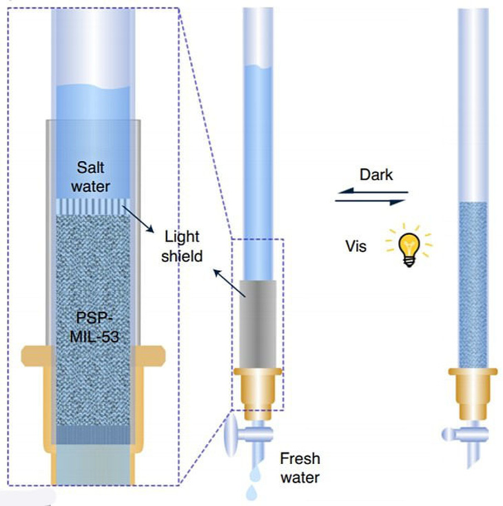
• Phương pháp lọc sử dụng ánh sáng mặt trời

Bộ lọc sử dụng các vật liệu khung hữu cơ - kim loại (MOFs), gồm các hợp chất chứa các ion kim loại hình thành một vật liệu tinh thể với bề mặt riêng lớn hơn mọi vật liệu từng được biết tới nay. Trong quá trình khử muối, bước đầu, một bộ lọc MOF chuyên dụng sẽ tách hoàn toàn muối từ nước biển, quy trình này không tiêu thụ năng lượng. Sau đó, bộ lọc MOF này sẽ được đưa ra dưới ánh nắng mặt trời trực tiếp trong chưa đầy 4 phút để tái tạo chức năng, trước khi được đưa trở lại để thực hiện quy trình tách muối thêm một lần nữa.

(Nguồn: https://tuoitre.vn/cong-nghe-loc-nuoc-bien-thanh-nuoc-uong-chi-trong-30-phut-202008121037464.htm)

 

Tham khảo

• https://khoahoc.vietjack.com/question/726111/nuoc-tren-trai-dat-phan-bo-chu-yeu-o-bien-va-dai-duong
• https://vnexpress.net/tai-sao-nuoc-tren-trai-dat-duoc-phan-bo-deu-4113087.html
• https://www.australianenvironmentaleducation.com.au/education-resources/what-is-water/
• https://dienmaysakura.vn/vong-tuan-hoan-nuoc.html
• https://www.intechopen.com/chapters/63043
• https://locnuocvietan.vn/loc-nuoc-bien-thanh-nuoc-ngot/